Database Fundamentals - Summary

1. Introduction to DBMS and Data Modeling Part I

1.1 Introduction to Database Concepts

1. Business Rules (BR)

• Business rules define the structure and constraints of a business scenario in a database context.

• They help identify:

  • Entities (e.g., Member, Book)
  • Attributes (e.g., Title, Author)
  • Relationships (e.g., a member can rent many books)
  • Identifiers (e.g., membership number as a unique ID)

2. Primary Key (PK)

• A Primary Key uniquely identifies each record in a table.
• Example: A student’s unique ID (e.g., student number).
• In ERDs, PKs are bolded and underlined.

3. Foreign Key (FK)

• A Foreign Key is a reference to a Primary Key in another entity.
• It establishes relationships between tables (e.g., Rentals refer to both Member and Book).
• In ERDs, FKs are implied by lines, not listed as attributes.

4. Entity Relationship Diagrams (ERD)

• Graphical representation of a database model.

• Composed of:

  • Entities: collections of related attributes (e.g., Book, Member, Rental)
  • Attributes: individual data fields (e.g., name, DOB)
  • Relationships: how entities relate (e.g., a member rents a book)

---

2. Structured Query Language (SQL) - Data Definition Language (DDL) and Data Manipulation Language (DML)

2.1 DDL and DML

• DDL commands: CREATE, ALTER, DROP, RENAME
• DML commands: INSERT, DELETE, UPDATE

1. Create Table and Constraints, and DROP

Defines the structure of a table, including columns and constraints.

CREATE TABLE Customer_T (
  CustomerID NUMERIC(4) NOT NULL,
  CustomerName VARCHAR(25),
  CustomerState CHAR(2),
  CONSTRAINT Customer_PK PRIMARY KEY (CustomerID)
);

A primary key constraint can be defined in two ways:

• Named constraint (out-of-line):
  • CONSTRAINT Customer_PK PRIMARY KEY (CustomerID)
  • This allows you to assign a custom name like Customer_PK, which is useful for clarity, maintenance, and future alterations
• Inline constraint:
  • CustomerID NUMERIC(4) NOT NULL PRIMARY KEY
  • This creates the constraint without a custom name. Instead, the database auto-generates a name.
  • Less readable and harder to reference

DROP table

DROP TABLE Customer_T

2. Insert Data

Adds new rows to a table.

-- With specific columns
INSERT INTO Customer_T (CustomerID, CustomerName, CustomerState)
VALUES (1, 'Contemporary Casuals', 'NSW');

-- Without specifying columns (must match column order)
INSERT INTO Customer_T
VALUES (2, 'Home Furnishings', 'VIC');

• Without specify columns: Data that will be insert must match with all columns.
• With specify columns: Only specific columns will be insert. Columns that aren't define will result as "(NULL)"

3. Update Data

Modifies existing data in a table.

UPDATE Customer_T
SET CustomerName = 'Modern Interiors'
WHERE CustomerID = 2;

4. Delete Data

Removes rows from a table.

DELETE FROM Customer_T
WHERE CustomerID = 2;

5. Alter Table

Modifies the structure of an existing table.

-- Add a column
ALTER TABLE Customer_T ADD CustomerEmail VARCHAR(100);

-- Drop a column
ALTER TABLE Customer_T DROP COLUMN CustomerEmail;

-- Rename a column
ALTER TABLE Customer_T RENAME COLUMN CustomerName TO Name;

-- Change data type
ALTER TABLE Customer_T ALTER COLUMN Name TYPE VARCHAR(50);

-- Set a default value
ALTER TABLE Customer_T ALTER CustomerState SET DEFAULT 'NSW';

-- Drop default
ALTER TABLE Customer_T ALTER CustomerState DROP DEFAULT;

-- Add a unique constraint
ALTER TABLE Customer_T ADD CONSTRAINT Unique_Name_Street
UNIQUE (CustomerName, CustomerState);

-- Rename the table
ALTER TABLE Customer_T RENAME TO Customer_Main;

6. Composite Keys

Combines multiple columns to form a single primary or foreign key.

CREATE TABLE OrderLine_T (
  OrderID NUMERIC(5) NOT NULL,
  ProductID NUMERIC(4) NOT NULL,
  OrderedQuantity NUMERIC(10),
  PRIMARY KEY (OrderID, ProductID), -- Composite PK (auto-named)
  FOREIGN KEY (OrderID) REFERENCES Order_T(OrderID), -- FK1 (auto-named)
  FOREIGN KEY (ProductID) REFERENCES Product_T(ProductID) -- FK2 (auto-named)
);

• Use constraint for set the name manually

CONSTRAINT OrderLine_PK PRIMARY KEY (OrderID, ProductID),
CONSTRAINT FK_Order FOREIGN KEY (OrderID) REFERENCES Order_T(OrderID),
CONSTRAINT FK_Product FOREIGN KEY (ProductID) REFERENCES Product_T(ProductID)

7. Design Reminders

Best practices when designing tables and relationships.

• Create primary key tables before foreign key tables.
• Foreign key columns must match the data type of the referenced primary key.
• Use domain constraints:

State CHAR(2) CHECK (State IN ('NSW', 'VIC', 'QLD', 'SA', 'WA', 'ACT', 'NT'))

• Use DEFAULT CURRENT_DATE for automatic dates.

8. Foreign Key with Default Value

Defines a foreign key and uses a default value for a column.

CREATE TABLE Order_T (
  OrderID NUMERIC(5) NOT NULL,
  CustomerID NUMERIC(4),
  OrderDate DATE DEFAULT CURRENT_DATE,
  PRIMARY KEY (OrderID),
  FOREIGN KEY (CustomerID) REFERENCES Customer_T(CustomerID)
);

9. Querying Relationships

Examples of retrieving data using PK–FK relationships.

-- Retrieve all data from table
SELECT * FROM Order_T;

-- Retrieve some fields from table
SELECT field-1, field-2 FROM Order_T;

-- Retrieve all orders for CustomerID 1, allow: =, >, <, <=, >=, and, or
SELECT * FROM Order_T WHERE CustomerID = 1;

-- Count how many orders a customer has placed
SELECT COUNT(*) FROM Order_T WHERE CustomerID = 1;

---

3. Data Modeling Part II

3.1 Modeling Relationships

Relationship

1. Relationship Types vs. Relationship Instances

• Relationship Type: General pattern showing how two or more entities are related (e.g., "Instructor teaches Subject").
• Relationship Instance: Specific example of the relationship in the database (e.g., "Fahimeh teaches Database Fundamentals").
• Relationship type appears as lines in an ERD; instances are rows in related tables.

Example

2. Degree of Relationships

• Degree: Number of entity types involved in the relationship.

  • Unary: One entity related to itself.
  • Binary: Two entities involved.
  • Ternary: Three entities involved.

Example

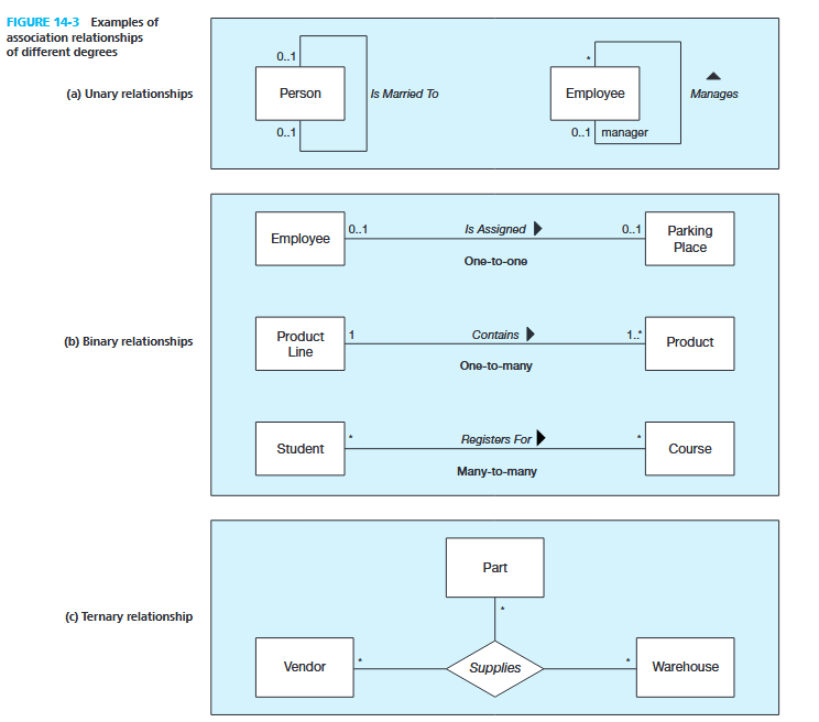
3. Cardinality of Relationships

• Cardinality: Number of entity instances that can or must be associated.

  • One-to-One (1:1): Each record relates to only one in the other table.
  • One-to-Many (1:M): One record relates to many others.
  • Many-to-Many (M:N): Many records relate to many others.

• Minimum cardinality: Optional (0) or mandatory (1+).

• Maximum cardinality: Maximum allowed links.

Example

4. Multiple Relationships Between Entities

• Two entities can have more than one type of relationship at the same time.
• Example: A professor can teach courses and also be qualified to teach other courses.
• May include additional rules, like minimum numbers.

Example

5. Relationships with Attribute(s)

• A relationship can have its own attributes.
• Example: "DateCompleted" in the relationship between Employee and Course.
• These attributes describe the association itself, not the entities.

Example

Associative Entity – Combination of Relationship and Entity

M:N Relationship -> Two 1:M relationships

• Converts an M:N relationship into two 1:M relationships.
  • Relational databases do not support M:N relationships directly.
  • Must break it down into two 1:M relationships using an associative entity
• Acts as both a relationship and an entity with attributes.
• Usually has a composite primary key from the related entities.

Example

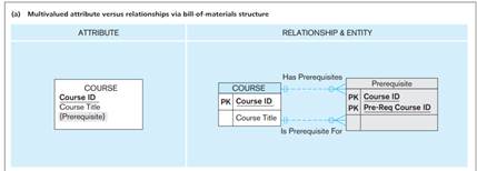
Multivalued Attributes Can be Represented as Relationships

Multivalued Attributes

• If an attribute can have multiple values, store it in a separate related table.
• Simple Multivalued Attributes:
  • 
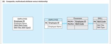
• Composite Multivalued Attributes:
  • 

Weak and Strong Entities – Identifying Relationship

• Strong Entity: Can exist independently; has its own PK.
• Weak Entity: Depends on a strong entity’s PK for identification; cannot exist without it.
• Identifying Relationship: Double line; connects strong to weak entity.
• Weak entity PK (Composite Key) = Strong entity PK + its own partial key.

Example

3.2 Notations

• Crow’s Foot Notation is commonly used in ERDs:
  • Boxes = Entities.
  • Lines = Relationships.
  • Symbols show cardinality (e.g., one, many).
• Solid line: Normal relationship.
• Double line: Identifying relationship (weak and strong entities).
• Attributes: Shown inside entity boxes; PKs underlined.

Example

---

4. Data Modeling Part III

4.1 Supertypes, Subtypes, Relationship

Supertypes and Subtypes

• Supertype: general entity with common attributes.
• Subtype: subgroup with distinct attributes or relationships.
• Attribute inheritance: subtypes inherit all supertype attributes.
• Rule: create subtypes only if specific attributes/relationships exist.
• PK of supertype = also PK (and FK) in each subtype.

Example Cases

Vehicles: CAR, TRUCK share attributes → VEHICLE supertype

Relationships and Subtypes

All subtypes share a relationship & Only some subtypes have unique relationships

• If all subtypes share a relationship → define at supertype level.
  • All PATIENT is cared for RESPONSIBLE PHYSICIAN
• If only some subtypes have unique relationships → define at subtype level.
  • RESIDENT PATIENT is (only) assigned to BED

Generalization vs Specialization

• Generalization (bottom-up): combine similar entity sets into a more general supertype
  • Car, Truck -> Vehicle
• Specialization (top-down): create subtypes from a supertype.
  • Top-down process: start from a supertype and define one or more subtypes that capture distinct attributes/relationships.

Specialization to MANUFACTURED PART and PURCHASED PART

• Example: PART specialized into MANUFACTURED PART and PURCHASED PART.
• Issues: multivalued attributes and data duplication → solved with associative entities (e.g., SUPPLIES linking PART and SUPPLIER).

Constraints in Supertype/Subtype Relationships

Disjoint vs Overlap and Total vs Partial Specialization

• Disjoint vs Overlap:
  • Disjoint (D): An entity can belong to only one subtype. Example: A Vehicle is either a Car or a Truck, not both.
  • Overlap (O): An entity can belong to multiple subtypes. Example: A Person could be both a Student and an Employee.
• Total vs Partial Specialization:
  • Total specialization (T): Every entity in the supertype must belong to at least one subtype. Example: Every Employee must be either a SalariedEmployee or an HourlyEmployee.
  • Partial specialization (P): Some entities in the supertype may not belong to any subtype. Example: A Vehicle may be a Car, or a Truck, or just a Vehicle with no subtype.

Completeness Constraint

Determines whether every instance of a supertype must belong to a subtype.

• Total Specialization (Double Line): Every supertype instance must be in at least one subtype.
  • 
• Partial Specialization (Single Line): Some supertype instances may not belong to any subtype.
  • 

Disjointness Constraint

Determines whether a supertype instance can belong to one or more subtypes at the same time.

• Disjoint Rule: A supertype instance can be a member of only one subtype.
  • 
• Overlap Rule: A supertype instance can belong to multiple subtypes.
  • 

Subtype Discriminator

An attribute of the supertype used to decide which subtype(s) an instance belongs to.

• Disjoint Case: A simple attribute with alternative values (e.g., Type = {Car, Truck}).
  • 
• Overlap Case: A composite attribute (set of Boolean flags) where each flag shows whether the instance belongs to that subtype (e.g., Is_Student = Y/N, Is_Employee = Y/N).
  • 
  • Example:
    • Employee_Type ∈ {H, S, C} tells us if EMPLOYEE is Hourly, Salaried, or Consultant
    • Example: H? S? C? with Y/N values.
    • YNY = employee is Hourly and Consultant.
    • NYN = employee is only Salaried.

---

5. Convert ERD to Relations

5.1 Relational Model

Components of relational model

• Data Structure: Tables (relations), rows, and columns.
• Data Manipulation: SQL operations (queries, inserts, updates).
• Data Integrity: Rules to maintain accuracy (primary key, foreign key, constraints).

Relations (Table)

• A relation = named table with rows and columns.
• Requirements to qualifty table as relation:
  • Unique table name.
  • Atomic attribute values (no multivalued/composite).
  • Unique rows.
  • Unique column names.
  • Order of rows/columns irrelevant.

Relational Model Concepts Correspond to E-R Model

Entity to Relation

• Relations (tables) correspond with entity types and with many-to-many relationship types.
• Rows correspond with entity instances and with many-to-many relationship instances.
• Columns correspond with attributes.

Entity types

Relations (tables)

Ins_ID	Ins_F_Name	Ins_L_Name
12548	Danna	Ramezani
45476	Ricky	Brown
14475	Jack	Cooper

Integrity Constraints

3 Types of Constraints

• Domain Constraint: Values in a column must come from the same domain (e.g., Student_ID must be 4-digit integer).
• Entity Integrity: PK must not be null.
• Referential Integrity: FK must match a valid PK value in another table.

Referential Integrity Rules (for deletes):

1. Restrict – prevent deleting parent if child rows exist.
2. Cascade – delete child rows automatically when parent is deleted.
3. Set-to-Null – set FK to null when parent is deleted (not allowed for weak/mandatory entities).

5.2 Transforming ERD into Relations

Mapping ERD to Relations

• Simple attributes → direct columns.
  • 
• Composite attributes → break into component columns.
  • 
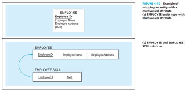
• Multivalued attributes → new table with FK back to main entity.
  • 

Mapping Binary Relationships

• 1:M → PK of “one” side becomes FK in “many” side.
  • 
• 1:1 → PK of mandatory side becomes FK in optional side.
  • 
• M:N → Create new relation (associative entity) with composite PK from both sides.
  • 

Mapping Ternary (and n-ary) Relationships

• 
• Create relation for each entity + one associative relation.
• Associative relation’s PK often includes multiple FKs (sometimes add surrogate key to simplify).

Mapping Weak Entities

• 
• Weak entity becomes its own table.
• PK = Partial identifier + PK of strong entity (as FK).
• FK cannot be null (mandatory).

Mapping Unary Relationships

• 
• 1:1 or 1:N → Recursive FK in the same table.
• M:N → Separate associative table with two FKs referencing same entity.

Mapping Supertype/Subtype Relationships

• One table for supertype, one for each subtype.
• Supertype PK = PK for subtypes.
• Discriminator attribute indicates subtype category.
• Subtype relations hold only their specific attributes.

---

6. Functional Dependencies, and Normalization

Week 5 Review "Relations":

• Show the primary key: Underline it (bold too if want)
• Have a composite primary key: Underline the entire key
• Show foreign keys: Asterisk*
• What if it’s a composite FK? (if the PK of the entity you’re getting it from is a composite PK): Put them around brackets, and asterisk*, Example: Prescription(DrugNo , (PatID,PatCID),Amount)

6.0 Key in Database

• Super Key: Any set of attributes that uniquely identifies a row.
  • Example: {StudentID}, {StudentID, Email}, {StudentID, Name, DOB}
• Candidate Key: Minimal super key (no unnecessary attributes).
  • Example: {StudentID}, {Email}
• Primary Key: Chosen candidate key that uniquely identifies rows. Must be unique and non-null.
  • Example: {StudentID}

6.1 Functional Dependencies

$\text{SubjectID} \implies \text{SubjectDuration, SubjectName}$

• Know the exact, specific, single VALUE of SubjectDuration, SubjectName if you know the VALUE of SubjectID
• Come from business rule and forms
• Values of Left Side uniquely identifies the values of the Right Side

Partial and Transitive Functional Dependencies

• Partial Functional Dependency: depends on part of a composite key.
  • Definition: When a non-key attribute depends on part of a composite primary key, not the whole key.
  • Example: OrderLine(OrderID, ProductID, Quantity, ProductName)
    • Primary Key = (OrderID, ProductID)
    • ProductName depends only on ProductID (part of the key). -> This is a partial dependency.
• Transitive Functional Dependency: depends on another non-key attribute.
  • Definition: When a non-key attribute depends on another non-key attribute, not directly on the primary key.
  • Example: Order(OrderID, CustomerID, CustomerName)
    • Primary Key = OrderID
    • CustomerName depends on CustomerID, which depends on OrderID. -> This is a transitive dependency.

6.2 Normalising Relation: 1NF, 2NF, 3NF

Normal Form

A relation is in 1NF (1st Normal Form) if

• Rule:
  • No repeating groups or multi-valued attributes.
  • Every attribute must be atomic (cannot be split further).
  • No derived attributes.
• Example (Not in 1NF):

STUDENT(StudentID, Name, Subjects)

• Subjects might store multiple values like {Math, Physics, English}. That breaks 1NF because Subjects is not atomic.
• Example (1NF):

STUDENT(StudentID, Name, Subject)

A relation is in 2NF (2nd Normal Form) if

• Rule:
  • Must already be in 1NF.
  • Remove Partial Dependencies
    • Partial Dependency: When you have dependencies on only PART of the PK
      • Can happen if you have a Composite PK (e.g. PatID, PatCID)
    • Every non-key attribute has to be fully functionally dependent on the ENTIRE primary key
• Example (Not in 2NF):
  • OrderDate depends only on OrderID.
  • ProductName depends only on ProductID.
  • These are partial dependencies.

ORDER_LINE(OrderID, ProductID, OrderDate, ProductName, Quantity)
PK = (OrderID, ProductID)

• Convert to 2NF:
  • Why: Splitting removes redundancy (e.g., product names repeated for every order line).

ORDER(OrderID, OrderDate)
PRODUCT(ProductID, ProductName)
ORDER_LINE(OrderID, ProductID, Quantity)

A relation is in 3NF (3rd Normal Form) if

• Rule:
  • Must already be in 2NF.
  • Remove transitive dependencies
    • Transitive Dependency: When you have dependency on a NON-KEY attribute.
    • We don't want functional dependencies on non-primary-key attributes
• Example (Not in 3NF):
  • DeptName depends on DeptID (a non-key attribute).
  • This is a transitive dependency.

EMPLOYEE(EmpID, EmpName, DeptID, DeptName)
PK = EmpID

• Convert to 3NF:
  • Why: Avoids repeating department names for every employee and keeps department data consistent.

EMPLOYEE(EmpID, EmpName, DeptID)
DEPARTMENT(DeptID, DeptName)

---

7. SQL I

7.1 Simple Query

Subject Context

• This lecture follows earlier weeks on ERD, keys, functional dependencies, and normalization.
• It introduces SQL, focusing on Data Manipulation Language (DML) with queries.

Objectives

• Understand and write simple SQL queries.
• Learn the structure and order of the SELECT statement.
• Use clauses: SELECT, FROM, WHERE, ORDER BY, GROUP BY, HAVING.
• Apply aggregate functions.
• Understand SQL processing order.
• Work with views.

The SELECT Statement

Structure

SELECT column1, column2
FROM table_name
WHERE condition
GROUP BY column1
HAVING condition
ORDER BY column1;

• SELECT → choose columns or expressions to return.
• FROM → specify tables or views.
• WHERE → filter rows.
• GROUP BY → categorize results.
• HAVING → filter groups (like WHERE, but for groups).
• ORDER BY → sort the results.

Examples

• SELECT * FROM product_t; → returns all rows and columns.
• SELECT productdescription, productfinish FROM product_t; → returns selected columns.

Eliminating Duplicates

• Use DISTINCT to remove duplicate values.

SELECT DISTINCT productfinish FROM product_t;

WHERE Clause

• Filters rows using conditions.

• Supports operators:

  • Comparison: =, >, <, >=, <=
  • Range: BETWEEN
  • Logical: AND, OR, NOT
  • Pattern matching: LIKE
  • Null checking: IS NOT NULL
  • Membership: IN

Examples:

• WHERE productstandardprice > 275
• WHERE productdescription LIKE '%Table'
• WHERE customerstate IN ('FL','TX','CA')

Boolean Logic

• Operator precedence:

  1. Parentheses ()
  2. NOT
  3. AND
  4. OR

• Parentheses can override default precedence.

ORDER BY

• Sort results ascending (ASC, default) or descending (DESC).
• Can sort by multiple columns.

ORDER BY customerstate ASC, customername DESC;

Aggregate Functions

• Summarize data.
• Common functions: AVG, SUM, MIN, MAX, COUNT.

Examples:

• SELECT AVG(productstandardprice) FROM product_t;
• SELECT COUNT(*) FROM product_t;

GROUP BY

• Groups rows by column(s) and applies aggregate functions.
• Rule 1: Columns in SELECT must also appear in GROUP BY (unless used with aggregates).
• Rule 2: Non-grouped columns must use aggregate functions.

Example:

SELECT customerstate, COUNT(customerstate)
FROM customer_t
GROUP BY customerstate;

HAVING

• Filters groups after aggregation.
• Example:

SELECT customerstate, COUNT(customerstate)
FROM customer_t
GROUP BY customerstate
HAVING COUNT(customerstate) > 1;

SQL Statement Processing Order

1. FROM
2. WHERE
3. GROUP BY
4. HAVING
5. SELECT
6. ORDER BY

Views

• Virtual tables created by queries.
• Dynamic View: Not stored on disk, always up to date, but slower.
• Materialized View: Stored on disk, faster but requires refresh.

Syntax:

CREATE VIEW ViewName AS
SELECT * FROM product_t;

7.2 Key Takeaways

• SQL queries are built using structured clauses.
• WHERE filters rows; HAVING filters groups.
• Aggregates summarize data, often with GROUP BY.
• Views provide simplified or customized data access.
• Always remember the processing order of SQL statements.

---

8. SQL II

8.1 Formula and Explanation

Diagram

Diagram of JOIN

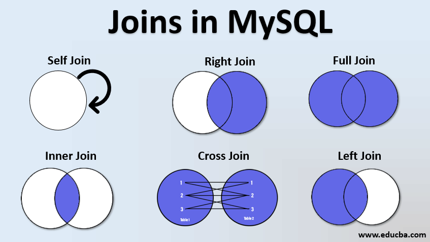
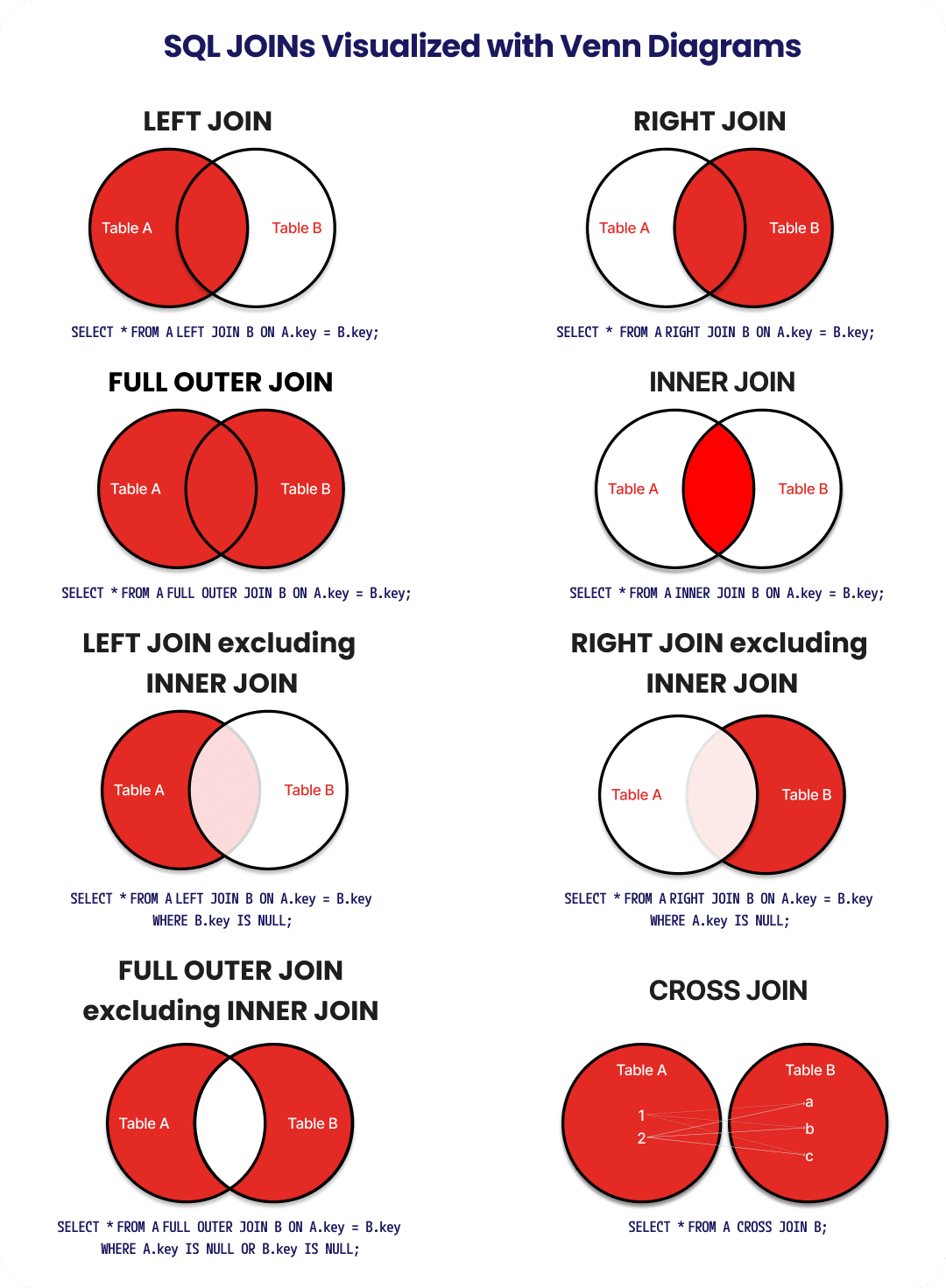
INNER JOIN

Formula:

SELECT *
FROM TableA
INNER JOIN TableB
ON TableA.col = TableB.col;

Explanation: Returns only rows where values match in both tables.

Example: Customers who have placed orders.

SELECT c.CustomerID, c.Name, o.OrderID
FROM Customer c
INNER JOIN Order o
ON c.CustomerID = o.CustomerID;

LEFT OUTER JOIN

Formula:

SELECT *
FROM TableA
LEFT JOIN TableB
ON TableA.col = TableB.col;

Explanation: All rows from the left table are returned. If there’s no match in the right table, NULL fills the missing values.

Example: Show all customers, even those with no orders.

SELECT c.CustomerID, c.Name, o.OrderID
FROM Customer c
LEFT JOIN Order o
ON c.CustomerID = o.CustomerID;

RIGHT OUTER JOIN

Formula:

SELECT *
FROM TableA
RIGHT JOIN TableB
ON TableA.col = TableB.col;

Explanation: All rows from the right table are returned, with NULL for missing left-side matches.

Example: Show all orders, even if some do not have a customer record.

SELECT c.CustomerID, c.Name, o.OrderID
FROM Customer c
RIGHT JOIN Order o
ON c.CustomerID = o.CustomerID;

FULL OUTER JOIN

Formula:

SELECT *
FROM TableA
FULL OUTER JOIN TableB
ON TableA.col = TableB.col;

Explanation: Returns all rows from both tables. Matches are combined; unmatched rows show NULL.

Example: Show all customers and all orders, matched where possible.

SELECT c.CustomerID, c.Name, o.OrderID
FROM Customer c
FULL OUTER JOIN Order o
ON c.CustomerID = o.CustomerID;

CROSS JOIN (Cartesian Product)

Formula:

SELECT *
FROM TableA
CROSS JOIN TableB;

Explanation: Pairs every row in the first table with every row in the second. Can generate very large results.

Example: Combine every customer with every product.

SELECT c.Name, p.ProductName
FROM Customer c
CROSS JOIN Product p;

2 style of queries for CROSS JOIN

1. Using CROSS JOIN

SELECT s1.stafName, s1.stalname, s1.staCSalary
FROM staff s1
CROSS JOIN staff s2
WHERE s2.staId = 'S632'
  AND s1.staCSalary > s2.staCSalary;

2. Using comma (old-style join syntax)

SELECT s1.stafName, s1.stalname, s1.staCSalary
FROM staff s1, staff s2
WHERE s2.staId = 'S632'
  AND s1.staCSalary > s2.staCSalary;

SELF JOIN

Formula:

SELECT e.EmployeeID, e.Name, m.Name AS Manager
FROM Employee e
INNER JOIN Employee m
ON e.ManagerID = m.EmployeeID;

Explanation: A table joins with itself using aliases. Useful for hierarchical data.

Example: Employees with their managers.

NATURAL JOIN (not recommended)

Formula:

SELECT *
FROM TableA
NATURAL JOIN TableB;

Explanation: Automatically joins on columns with the same name. Can cause unexpected results. Explicit INNER JOIN is safer.

UNION

Formula:

SELECT col1, col2 FROM TableA
UNION
SELECT col1, col2 FROM TableB;

Explanation: Combines the results of two queries. Removes duplicates unless UNION ALL is used.

Example: List all customer IDs from two different tables.

SELECT CustomerID FROM OnlineCustomer
UNION
SELECT CustomerID FROM StoreCustomer;

---

9. SQL III

9.1 Subquery

Subquery definition

• A subquery is a query inside another query. Also called nested queries.

• Only appear inside from below clauses:

  • FROM → acts like a temporary table.
  • WHERE → used as a condition.
  • HAVING → used to filter groups.

• Types of subqueries

  • Uncorrelated (simple) → runs once, result is reused by the outer query.
  • Correlated (advanced, next week) → runs once for every row in the outer query.

Example of Subquery

• SQL runs the innermost subquery first, then moves outward.
• Example:

SELECT ProductName
FROM ProductTable
WHERE ProductPrice = (SELECT MAX(ProductPrice) FROM ProductTable);

• Step 1: Find highest price.
• Step 2: Use that number in the outer query to return the product.

Subquery operators

• When a subquery returns multiple values, special operators are needed:

  • IN → checks if a value is in the list (X IN (subquery))
  • ANY → true if at least one value matches (X = ANY (subquery))
  • ALL → must match all values (X >= ALL (subquery))

• Rules to remember:

  • IN = ANY
  • NOT IN = <> ALL
  • ALL/ANY work with comparisons (<, >, =), but IN does not.

Subquery vs. JOIN

• Use a JOIN → when you need columns from multiple tables at the same time.
• Use a subquery → when you want to filter using conditions, or find max/min.
• Subqueries are often simpler and more efficient, but not always.

What should you take away from Week 9?

• By the end of this week, you should know:
  • ✅ What an uncorrelated subquery is.
  • ✅ Which parts of a query (FROM, WHERE, HAVING) can contain subqueries.
  • ✅ How to handle subqueries that return more than one row (using IN, ANY, ALL).
  • ✅ The execution order (inside → out).
  • ✅ When to use a subquery vs. join.

---

10. SQL IV

10.1 Correlated Subqueries

Definition

• A correlated subquery is a subquery that depends on data from the outer query.
• Unlike a simple (uncorrelated) subquery, which runs once and reuses its result, a correlated subquery executes once for every row in the outer query.

Purpose

• Correlated subqueries are used when each row of the main query requires a different calculation or comparison.
• Such as comparing each staff member’s salary with the average salary in their own state.

Example Comparison:

1. Show all staff with a salary above the average staff salary → uses a simple subquery (same average for all).
2. Show all staff with a salary above the average salary for the state where they live → uses a correlated subquery (average differs by state).

Step-by-Step Construction

Example: Show all staff with a salary above the average for their state.

1. Alias the outer table

   SELECT StaFName, StaLName, StaSalary, StaState  
   FROM Staff S1

   • The alias S1 allows the outer table to be referenced inside the subquery.

2. Create a simple subquery

   WHERE StaSalary > (SELECT AVG(StaSalary) FROM Staff)

   • Calculates one overall average (not yet correlated).

3. Add correlation (reference outer table)

   WHERE StaSalary > (SELECT AVG(StaSalary)  
                      FROM Staff  
                      WHERE StaState = S1.StaState)

   • The subquery now recalculates the average salary for each state by using S1.StaState from the outer query.

Full example of correlated subqueries

SELECT 
    StaFName, 
    StaLName, 
    StaSalary, 
    StaState
FROM 
    Staff S1
WHERE 
    StaSalary > (
        SELECT AVG(StaSalary)
        FROM Staff
        WHERE StaState = S1.StaState
    );

How It Works

• The SQL engine processes each row in the outer table.
• For each row, it substitutes that row’s state (e.g., 'VIC') into the subquery and calculates the average salary for that state.
• The comparison checks if the staff member’s salary is above the state’s average.
• This process repeats for every row.

Example Result: Only staff with salaries higher than their state’s average are returned.

StaFName	StaLName	StaSalary	StaState
Jordan	Tuckson	170000	VIC