41128 - Summary

1. Introduction to Software Analysis and Verification

1.1 Main question and Purpose

Week 1 - 3

Purpose

• Main question
  • Why do we need software analysis?
• Large programs can contain problems such as:
  • memory leaks
  • buffer overflows
  • uninitialised variables
  • use-after-free errors
  • security vulnerabilities
• It is difficult for developers to manually examine every possible path in a program containing thousands or millions of lines.
• Software analysis therefore uses algorithms and tools to automatically reason about program behaviour.

1.2 Static analysis versus dynamic analysis

Static analysis	Dynamic analysis
Examines code without running it	Examines the program while it runs
Attempts to consider all possible paths	Only observes paths executed by the test inputs
Can find problems before deployment	Finds problems that actually occur during execution
May produce false alarms	May miss untested problems
Used heavily in this subject	Examples include testing, fuzzing and sanitizers

• A helpful way to remember this:
  • Static: “What might happen?”
  • Dynamic: “What happened during this execution?”

1.3 Software analysis versus software verification

• The slides distinguish them by their goal:
  • Software analysis: tries to find whether a bug may exist.
  • Software verification: tries to prove that a program satisfies its specification and that certain bugs cannot occur.

For example:

assert(x > 0);

The assertion is a small specification saying:

“Whenever execution reaches this line, x must be greater than zero.”

A static verification tool attempts to determine whether this assertion can ever fail without actually running the program.

The two larger subject projects

Project 1: Static taint checker

It tracks untrusted information from a source to a sink.

It needs:

1. C/C++ programming
2. LLVM IR
3. graph representations
4. control-flow analysis
5. data-flow analysis
6. taint-path detection and visualisation

Project 2: Static symbolic execution

It reasons about possible values and program conditions to determine whether assertions can fail.

It needs:

1. LLVM IR and code graphs
2. control-flow reachability
3. constraint generation
4. a constraint or assertion solver

---

2. LLVM and SVF

Purpose of 2A and 2B

Purpose 2A

• Main question
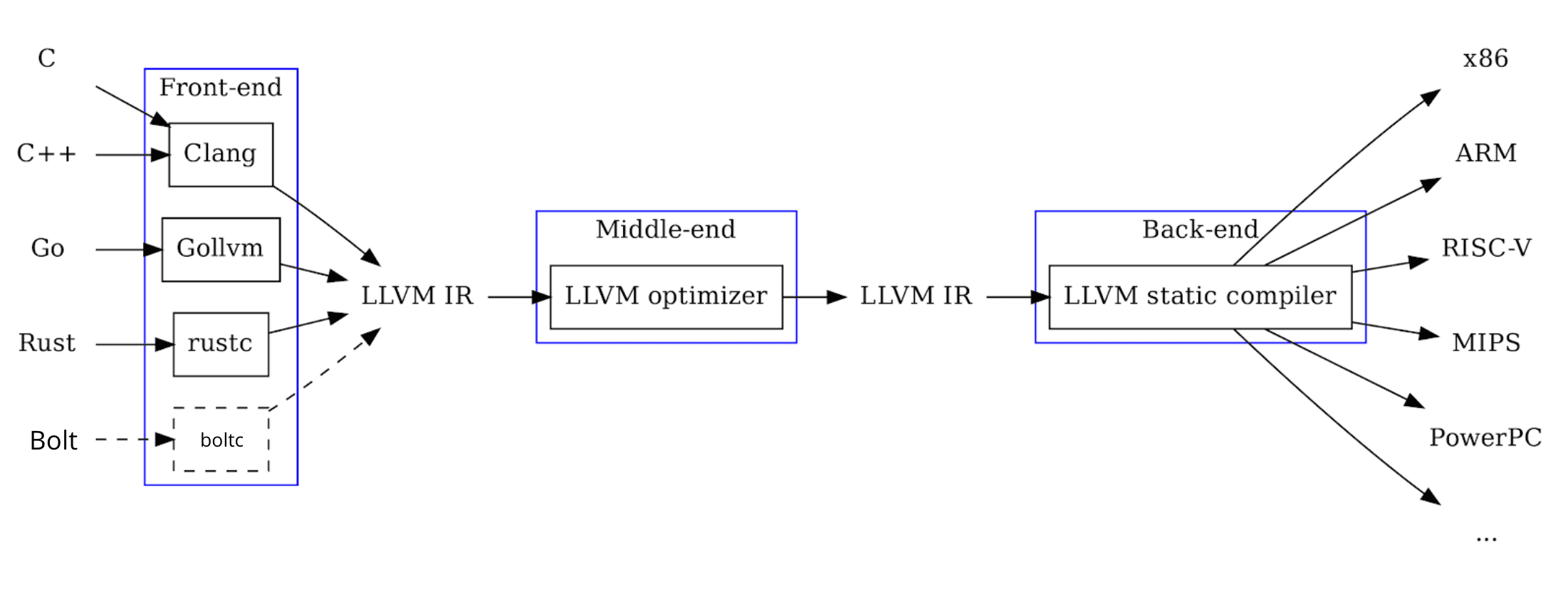
  • How can an analysis tool understand C or C++ code consistently?
  • Directly analysing source code is difficult because source languages contain many complicated constructs.
  • Therefore, Clang translates C/C++ into a simpler, standard representation called LLVM Intermediate Representation, or LLVM IR.

Purpose 2B

• Main question
  • How do we turn LLVM instructions into structures that analysis algorithms can easily use?
• LLVM IR is more manageable than C++, but it still contains many instruction types and compiler details.
• SVF provides another abstraction called SVFIR:

LLVM IR → SVFIR → code graphs → analysis algorithms

• SVFIR is built from LLVM IR. It does not independently replace LLVM IR.

2A. LLVM Compiler and LLVM IR

What is LLVM IR?

LLVM IR is:

lower-level than C/C++ higher-level than machine code strongly typed language-independent structured into modules, functions, basic blocks and instructions designed to support compiler optimisation and program analysis

For example, a source-code expression:

a = b + c * d;

might be separated into simpler instructions:

t = c * d
a = b + t

Each instruction performs a small operation. That makes relationships between values easier for an analysis tool to follow.

Static Single Assignment — SSA

LLVM IR generally uses Static Single Assignment form.

It means each LLVM variable is assigned only once.

Normal code:

x = 1;
x = x + 2;

SSA-style representation:

x1 = 1
x2 = x1 + 2

LLVM IR Scopes and Identifier

1. LLVM IR structure and scopes

Module
├── Global variables
└── Functions
    ├── Arguments
    └── Basic blocks
        └── Instructions

---

• Module
  • A module represents one complete LLVM IR file or compilation unit.
  • It contains:
    • Global variables
    • Function definitions
    • Function declarations

Example

@counter = global i32 0

define i32 @main() {
    ret i32 0
}

Here, @counter and @main belong to the module.

---

• Function
  • A function contains:
    • Function parameters
    • One or more basic blocks
    • Local identifiers used by its instructions

define i32 @add(i32 %x, i32 %y) {
entry:
    %result = add i32 %x, %y
    ret i32 %result
}

• In this example:
  • @add is the function.
  • %x and %y are arguments.
  • entry is a basic block.
  • %result is a local identifier.

---

• Basic block
  • A basic block is a continuous sequence of instructions.
  • A basic block:
    • Has one entry point
    • Runs instructions from top to bottom
    • Ends with a terminating instruction such as ret, br, or switch

entry:
    %result = add i32 %x, %y
    ret i32 %result

• Both instructions belong to the entry block.

2. LLVM identifiers: @ versus %

• LLVM uses prefixes to show the scope of an identifier.

Prefix	Meaning	Scope	Examples
@	Global identifier	Entire module	@main, @swap, @counter
%	Local identifier	Current function	%a, %b, %result
No prefix with :	Basic-block label	Current function	entry:, if.then:

---

• Global identifiers: @
  • Functions and global variables normally use @.

@number = global i32 10

define i32 @main() {
    ret i32 0
}

• @number is a global variable.
• @main is a global function name. They can be referenced from other functions in the module.

---

• Local identifiers: %
  • Function parameters and instruction results use %.

define i32 @double(i32 %value) {
entry:
    %result = mul i32 %value, 2
    ret i32 %result
}

• %value and %result only exist inside @double.
• Another function may also have a %result; this is allowed because each function has its own local scope.

Common LLVM IR instructions

• You do not need to memorise the entire LLVM language, but you should recognise: | LLVM instruction | Simplified meaning | | ---------------- | ------------------------------------------------- | | alloca | Create stack storage | | load | Read from memory | | store | Write to memory | | call | Call a function | | ret | Return from a function | | br | Branch to another basic block | | icmp | Compare integer values | | phi | Combine values arriving from different paths | | getelementptr | Calculate the address of a field or array element |

2B. SVFIR and Code Graphs

Main question and What is SVFIR?

Main question

• Main question
  • How do we turn LLVM instructions into structures that analysis algorithms can easily use?
• LLVM IR is more manageable than C++, but it still contains many instruction types and compiler details.
• SVF provides another abstraction called SVFIR:

LLVM IR → SVFIR → code graphs → analysis algorithms

• SVFIR is built from LLVM IR. It does not independently replace LLVM IR.

What is SVFIR?

SVFIR = SVFValue + SVFVar + SVFStmt + Code Graphs

• In simpler language:
  • SVFValue: wrapper around an LLVM value
  • SVFVar: a program variable or memory object
  • SVFStmt: a relationship or operation between variables
  • Code graph: puts those items into a graph that an algorithm can traverse
• SVFIR simplifies complicated LLVM operations into a smaller number of analysis-friendly statements.

Important SVF statements

SVF statement	Simplified meaning
AddrStmt	p = &object
CopyStmt	p = q
LoadStmt	p = *q
StoreStmt	*p = q
GepStmt	Address of an array element or structure field
PhiStmt	Value comes from one of several paths
BranchStmt	Conditional control flow
CallPE	Pass actual arguments into function parameters
RetPE	Pass a returned value back to the caller

The three most important graphs: "Call Graph", "Control-Flow Graph and ICFG", "Program Assignment Graph — PAG"

1. Call Graph

A call graph provides a function-level view.

• Node = function
• Edge = one function may call another

---

• It answers:
  • “Which functions can call which other functions?”
• It does not show every statement inside the functions.

2. Control-Flow Graph and ICFG

• A CFG describes the possible execution order of statements inside one function.
• An Interprocedural Control-Flow Graph, or ICFG, connects control flow across functions.
  • Node = instruction or statement
  • Edge = possible next execution step
• It answers:
  • “Can execution move from statement A to statement B?”

The ICFG is the graph used in Week 3.

3. Program Assignment Graph — PAG

• The PAG represents relationships between variables and memory objects.
  • Node = variable or memory object
  • Edge = assignment, load, store, address relationship, etc.
• It helps answer:
  • “How can a value move from one variable or memory location to another?”

The PAG becomes particularly important for data-flow and pointer analysis.

---

3. Control Flow and Interprocedural Analysis

3.1 Main question and Purpose

Purpose

• Main question
  • Where can program execution go?
• Before analysing data, we need the possible execution paths through a program.

3.2 Control Flow Graph (CFG)

A CFG represents possible execution paths inside one function.

• Node = instruction or basic block
• Edge = possible execution transition

For example:

if (x > 0)
    y = 10;
else
    y = 20;

print(y);

3.3 Intra-procedural versus interprocedural analysis

Intra-procedural	Interprocedural
Stays inside one function	Crosses function boundaries
Uses a CFG	Needs a call graph and an ICFG
Enough for local control flow	Needed for real programs that call other functions

Intra-procedural

Interprocedural

3.4 Call Graph

A call graph shows which functions may call other functions. Week 2B already introduces it as the function-level view. Week 3 uses it for interprocedural analysis.

It answers:

• “Which functions can call which other functions?”

For example:

main() {
    foo();
}

foo() {
    bar();
}

Indirect calls

Sometimes the target is not obvious:

fp();

If pointer analysis determines pts(fp) = {foo, bar}, the possible call targets are:

3.5 ICFG

ICFG = Interprocedural Control Flow Graph.

It extends control-flow analysis across functions.

main() {
    foo();
}

Important SVF ICFG nodes:

Node	Purpose
FunEntryICFGNode	Function entry
FunExitICFGNode	Function exit
CallICFGNode	Function call
RetICFGNode	Return site
IntraICFGNode	Normal instruction

• Key takeaway
  • CFG → control flow inside a function
  • Call graph → relationships between functions
  • ICFG → detailed control flow across functions

---

4. Data Dependence and Pointer Analysis

4.1 Main question and Purpose

Purpose

• Main question
  • Where can data go?
• Week 3 asked where execution can go. Week 4 asks how values move, especially through pointers and memory.

For example:

x = 10;
y = x;

There is a data dependence because y uses the value defined by x:

4.2 Why pointers make data dependence difficult

*p = 50;
x = *q;

Does x depend on the first statement? We do not know until we know whether p and q could point to the same memory.

If p and q both point to A:

then the store through p can affect the load through q, so there is a possible data dependence.

4.3 Pointer basics

int a = 10;
int *p = &a;

Expression	Meaning
a	value of a
&a	address of a
p	address stored in p
*p	value at the address p points to

• Therefore:
  • a and *p are values
  • &a and p are addresses

4.4 The four important pointer operations

Code	Operation	Meaning
p = &a	Address	p points to a
q = p	Copy	copy address from p to q
q = *p	Load	read the value or pointer stored through p
*p = q	Store	write a value or pointer through p

• Easy memory rule
  • p = &a → address
  • q = p → copy address
  • q = *p → read / load
  • *p = q → write / store

q = p versus q = *p

int a = 10;
int *p = &a;

Copy copies the address:

int *q = p;

Both p and q point to a.

Load copies the value:

int q = *p;

So:

• q = p → copy address
• q = *p → read value

Store

int a = 10;
int *p = &a;
int q = 50;

*p = q;

Because p points to a, *p = q means a = q.

• Before: p → a = 10, q = 50
• After: p → a = 50, q = 50

4.5 Points-to sets and alias analysis

A points-to set contains the possible memory objects a pointer may reference.

• pts(p) = {a} means p may point to a.
• pts(p) = {a, b} means p may point to a or b.

Two pointers may alias if they may reference the same memory object.

If:

• pts(p) = {A, B}
• pts(q) = {B, C}

then pts(p) ∩ pts(q) = {B}, so they may alias.

• General rule
  • If pts(p) ∩ pts(q) ≠ ∅, they may alias.
• This helps determine whether a store through one pointer can affect a load through another.

4.6 PAG / SVFIR

The Pointer Assignment Graph (PAG) / SVFIR represents pointer and value constraints. Week 2B already introduces the PAG; Week 4 uses it for pointer analysis.

p = &a;
q = p;

After pointer analysis:

• pts(p) = {a}
• pts(q) = {a}

Therefore p and q may alias.

4.7 Andersen's pointer analysis

Andersen analysis calculates what each pointer can possibly point to.

It processes the constraints in the PAG / SVFIR and propagates points-to information.

p = &a;
q = p;
r = q;

• Start
  • pts(p) = {a}
  • pts(q) = {}
  • pts(r) = {}
• Propagate along p → q → r
• Final
  • pts(p) = {a}
  • pts(q) = {a}
  • pts(r) = {a}

Flow insensitivity

Classic Andersen analysis is flow-insensitive.

p = &a;
q = &b;

r = p;
r = q;

At actual runtime, r = p makes r point to a, then r = q overwrites that, so r ends pointing to b.

Andersen generally collects both possibilities:

• pts(r) = {a, b}

because it does not distinguish statement order in its overall points-to result. It says: somewhere in the analysed program, r may receive the address of a or b.

4.8 Fixed point

Andersen repeatedly propagates information until nothing new can be added.

When nothing new can be added, it has reached a fixed point.

4.9 Week 4 summary

Week 4’s purpose is to determine how values can flow, especially through pointers and memory.

---

5. Information Flow Tracking and Taint Analysis

5.1 Main question and Purpose

Purpose

• Main question
  • Can a particular piece of information flow from a source to a sink?
• Week 5 combines Weeks 3 and 4. This is information-flow tracking.

5.2 Source, tainted data, and sink

A source is where interesting or untrusted data originates.

Examples include user input, network input, file input, and environment data.

x = getUserInput();

If getUserInput() is a source, x becomes tainted.

Tainted data is data originating from a source that we want to track.

x = source();
y = x;
z = y;

A sink is a sensitive operation where tainted data may be dangerous.

Examples include SQL execution, OS command execution, file operations, and network output.

system(x);

If a valid flow from source to sink exists, the analyser may report a potential vulnerability.

Simple taint analysis

x = source();
y = x;
sink(y);

Therefore the source can reach the sink.

5.3 Why Weeks 3 and 4 are needed

Why Week 4 is needed

Pointers hide data movement through memory:

int input = source();

int a;
int *p = &a;
int *q = p;

*p = input;

int x = *q;

sink(x);

Week 4 determines:

• pts(p) = {a}
• pts(q) = {a}

so p and q alias. Week 5 can then find:

Without pointer analysis, the analyser may not know that the store through p can affect the load through q.

Why Week 3 is needed

Real programs contain function calls.

void process(int x) {
    sink(x);
}

int main() {
    int input = source();
    process(input);
}

Week 3’s call graph and ICFG tell us how execution moves between these functions.

5.4 Context sensitivity

Suppose the same function is called multiple times:

foo(tainted);
foo(safe);

A context-sensitive analysis remembers which call led into the function.

• Correct
  • Call A → foo → return A
  • Call B → foo → return B
• Incorrect
  • Call A → foo → return B

The incorrect matching creates an impossible execution path and may cause false positives.

Call stack

Context can be understood using a stack.

main() {
    foo();
}

foo() {
    bar();
}

• Call foo → stack [foo]
• foo calls bar → stack [foo, bar]
• bar returns → [foo]
• foo returns → []

This helps match calls with their correct returns.

5.5 SVFG

SVFG = Sparse Value-Flow Graph.

It represents relevant value-flow relationships:

• Where was a value defined?
• Where can that value flow?
• Where can it be used?

The SVFG lets analyses such as taint analysis traverse value-flow paths.

Direct versus indirect value flow

Direct:

x = source();
y = x;

Indirect through memory:

*p = x;
y = *q;

If Week 4 determines that both p and q point to A:

This is an indirect memory-based flow.

5.6 Analysis process

A simplified taint-analysis process:

For interprocedural analysis, the traversal must also respect valid call/return contexts.

5.7 Connecting Weeks 3, 4 and 5

	Week 3	Week 4	Week 5
Focus	Control flow	Data dependence	Information flow
Question	Where can execution go?	Where can data and pointers go?	Can source reach sink?
Main graph	CFG / ICFG	PAG / SVFIR	SVFG
Important analysis	Interprocedural analysis	Andersen pointer analysis	Taint analysis
Key concepts	Call, return, entry, exit	Points-to, alias, load/store	Source, sink, taint
Purpose	Find valid execution paths	Find data dependencies	Find security / information flows

• One sentence per week
  • Week 3: find the possible execution paths through and between functions.
  • Week 4: find how data and pointers relate, including hidden memory dependencies caused by aliasing.
  • Week 5: use those relationships to determine whether specific information can flow from a source to a sink.

5.8 Complete example

void process(int *q) {
    int x = *q;
    sink(x);
}

int main() {
    int input = source();
    int a;
    int *p = &a;
    *p = input;
    process(p);
}

Week 3 — Control flow

Execution can reach process() and the sink.

Week 4 — Data dependence

int *p = &a;

gives pts(p) = {a}. When p is passed to process, q can point to the same object:

Therefore:

Week 5 — Information flow

There is a valid source-to-sink information flow.

---

6. Program Verification Against Software Vulnerabilities

6.1 Main question and Purpose

Purpose

• Main question
  • What real software vulnerabilities can happen, why they happen, and what conditions should be checked to prevent them?
• The lecture groups vulnerabilities into memory-safety errors, arithmetic errors, tainted-input problems, injection problems, and side-channel attacks.
• The slides repeatedly use assertions to check important safety conditions before continuing execution.

6.2 Memory leak

A memory leak occurs when dynamically allocated memory is not freed along a program execution path.

List *list = new List();

If the program never properly deletes all allocated memory, the leak remains.

• Why it matters
  • Over time, the program may consume more and more memory.
• Secure idea
  • Make sure every allocated object is eventually freed.

Relation to Week 3

Memory leaks depend on execution paths. Week 3 asks where execution can go.

Control-flow analysis can help determine whether there is some path where allocated memory is never released.

6.3 Null pointer dereference

A null-pointer dereference happens when the program dereferences a pointer whose value is NULL or nullptr, often causing a crash.

Student* student = findStuRecord(id);

printf("%s", student->name);

findStuRecord() may return nullptr. Then student->name tries to access memory through an invalid pointer.

• Secure idea
  • Check before dereferencing:

assert(student != nullptr);

Relation to Week 4

Week 4 asks what a pointer can point to. Week 6 adds: is the pointer valid before we dereference it?

Week 4’s pointer analysis is directly useful here.

6.4 Dangling pointer / use-after-free

A dangling pointer is a pointer that no longer refers to a valid memory object, often because that object has already been freed.

char *ptr = malloc(SIZE);

free(ptr);

logError(ptr);

After free(ptr), the memory object is gone. Using ptr again is use-after-free.

• Secure idea
  • A defensive pattern shown in the lecture is:

free(ptr);
ptr = nullptr;

Relation to Week 4

Week 4 understands ptr → object A. Week 6 adds object lifetime:

Knowing where a pointer points is not enough; we also care whether the object still exists.

6.5 Buffer overflow

A buffer overflow occurs when the program writes more data than a buffer can hold and overwrites adjacent memory.

char *p = malloc(n);
int y = n;

p[y] = 'a';

If the buffer has n elements, valid indexes are 0 ... n-1. p[n] is outside the allocated area.

• Secure idea
  • Check the index before writing:

assert(y < n);

Relation to Weeks 3 and 4

• Week 3 helps determine whether execution can reach the dangerous access.
• Week 4 helps reason about the memory object being accessed.
• Week 6 asks: is the actual memory access valid?

6.6 Integer overflow

An integer overflow occurs when a calculation produces a value outside the range that the integer type can represent.

Easy definition: the result is too large to fit inside the integer type.

For unsigned integers, the lecture shows wrap-around behaviour:

• UINT_MAX + 1 = 0
• UINT_MAX + 2 = 1
• UINT_MAX + 3 = 2

Why it is dangerous

size = nresp * sizeof(char*);

If the real result is huge but the multiplication overflows:

The lecture gives an OpenSSH example where multiplication overflow leads to a heap buffer overflow.

• Secure idea
  • Check the value before the dangerous arithmetic or allocation:

assert(nresp <= userDefinedSize / sizeof(char*));

The lecture recommends checking the size before allocation.

6.7 Division by zero

A division-by-zero error occurs when the divisor becomes zero.

return totalTime / numRequests;

If numRequests = 0, the operation is invalid.

• Secure idea

assert(numRequests > 0);

before performing the division.

6.8 Tainted information flow

Tainted data means data that comes from an untrusted source, such as user or network input.

Week 6 explains that malicious input can cause unexpected behaviour, information leakage, or attacks.

char *pMsg = packet_get_string();

ParseMsg((LOGIN_MSG_BODY *)pMsg);

The lecture example shows attacker-controlled data influencing a loop bound and recommends checking it against a safe limit.

Relation to Week 5

This is a direct continuation of Week 5.

Week 5 tracks SOURCE → taint → value flow → sink.

Week 6 asks: what vulnerability can occur if that tainted value reaches an unsafe operation?

6.9 Code injection

Code injection happens when input that should only be treated as data becomes part of executable code or a command.

cin >> user_id;

system(command + user_id);

Expected: user_id = "05" produces cat user_info/05. If malicious command syntax is included in the user input, system() may execute unintended commands. The lecture identifies lack of validation before system() as the problem.

• Secure idea
  • Validate the input before passing it to system().
  • The lecture checks that the user ID contains numeric input before execution.

Relation to Week 5

This is another source-to-sink problem:

• Week 5 detects: tainted flow → system()
• Week 6 interprets: possible code injection

6.10 Format string vulnerability

A format string vulnerability occurs when user input is interpreted as formatting instructions rather than ordinary data.

Easy definition: user-controlled data becomes printf instructions.

Safe:

printf("%s", userInput);

• "%s" → format
• userInput → data

Vulnerable:

printf(userInput);

Now userInput is treated as format instructions. If the user provides %s%s%s%s, printf() may interpret those sequences as instructions to read string arguments that were never supplied. This can cause invalid memory access or a crash.

Relation to Week 5

6.11 SQL injection

SQL injection happens when user input is directly combined into an SQL query and changes the query’s meaning.

txtUserId = getRequestString("UserId");

txtSQL =
    "SELECT * FROM Users WHERE UserId = "
    + txtUserId;

The slides show that specially crafted input can modify the condition so that the database returns unintended records.

Relation to Week 5

SQL injection is another practical consequence of unsafe information flow.

6.12 Side-channel / timing attack

A side-channel attack occurs when secret information leaks through some observable program behaviour rather than through normal program output.

A timing attack uses how long the program takes as the observable information.

for (...) {
    if (guess[i] != password[i])
        return false;
}

Suppose the password is CAT123. An attacker may infer that more characters are correct because the program takes longer before returning:

• XXXXXX → fails quickly
• CXXXXX → slightly slower
• CAXXXX → even slower
• CATXXX → slower again

• Secure idea
  • Compare all characters instead of returning immediately:

for (i = 0; i < length; i++)
    result &= (ca[i] == cb[i]);

The goal is a constant-time comparison for a fixed input length.

Relation to Week 5

Week 5 mainly studies explicit value flow: variable → variable → sink.

Timing attacks show that information can also escape indirectly:

This extends information flow beyond normal data-flow edges.

6.13 Role of assertions

Assertions state: this condition must be true before continuing.

assert(student != nullptr);
assert(y < n);
assert(numRequests > 0);
assert(nresp <= safeLimit);

The important idea is not just the word assert, but the safety condition being checked.

6.14 Connecting Weeks 3–6

Week	Main question	How Week 6 uses it
Week 3	Where can execution go?	Find paths that reach dangerous operations or miss cleanup
Week 4	Where can pointers / data go?	Understand memory objects, pointer accesses and aliases
Week 5	Can information flow from source to sink?	Track tainted input into dangerous operations
Week 6	What vulnerability can happen?	Identify real bugs and the safety checks needed

Week 3 → Week 6

Week 3 gives the paths. Week 6 identifies a memory leak.

Week 4 → Week 6

Week 4 understands p → memory A. Then:

free(p);
*p = 10;

Week 6 identifies use-after-free.

Week 5 → Week 6

input = source();
system(input);

Week 5 finds SOURCE → input → SINK. Week 6 interprets the unsafe tainted flow as code injection.

6.15 Cheat sheet

Vulnerability	Remember
Memory leak	Allocated memory is never freed
Null dereference	Use *p when p == nullptr
Use-after-free	Use memory after it has been freed
Buffer overflow	Write outside buffer bounds
Integer overflow	Number does not fit its integer range
Division by zero	Divisor becomes 0
Tainted information flow	Untrusted data travels through the program
Code injection	User data becomes executable command or code
Format string	User data becomes printf instructions
SQL injection	User input changes an SQL query
Timing attack	Secrets leak through execution time

Weeks 3–5 teach you how to follow program execution and data. Week 6 uses that knowledge to recognise unsafe program behaviour and software vulnerabilities.

---

7. Code Verification and Predicate Logic

7.1 Main question and Purpose

Purpose

• Main question
  • Given a pre-condition and a program, can we prove that a safety assertion always holds?
• Weeks 3–6 analyse what a program can do. Week 7 checks whether what it does is correct / safe.
• The slides take program paths and SVF statements, translate them into logical formulas, and check each path.

Week	Main question	Connection to Week 7
Week 3 — Control flow	Where can execution go?	Gives the program paths that can be checked
Week 4 — Data dependence	Where can data / pointers go?	Gives relationships between values along those paths
Week 5 — Information flow	Can data flow from source to sink?	Identifies important flows that may need verification
Week 6 — Vulnerabilities	What can go wrong?	Introduces safety conditions such as assert(index < size)
Week 7 — Verification	Can we prove the safety condition holds?	Converts paths + assertions into logic and checks them

7.2 Formal verification

Formal verification means proving whether code satisfies a given specification using mathematical logic.

The lecture describes this as translating the specification and implementation into logical formulas, then using theorem-proving tools to check them.

7.3 Specification: pre-condition and post-condition

In this subject, specifications are embedded in the source code using assume and assert. The slides express this with Hoare logic:

P { prog } Q

Part	Meaning
P	Pre-condition — assumption before the program
prog	Program being checked
Q	Post-condition — assertion that should hold afterward

assume(x > 0);    // P

y = x + 1;        // program

assert(y > 0);    // Q

If x > 0 before execution, running the program should guarantee y > 0.

7.4 Main verification question

Week 7 asks:

Given the pre-condition and the program, will the assertion always hold?

assume(100 > x && x > 0);

if (x > 10) {
    y = x + 1;
}
else {
    y = 10;
}

assert(y >= x + 1);

Here:

• P = 100 > x > 0
• Q = y >= x + 1

7.5 Check each program path

This is where Week 3 control flow becomes important. The example has two paths:

Path 1

x > 10
y = x + 1

Assertion: y >= x + 1

Because y = x + 1, the assertion holds on this path.

Path 2

x <= 10
y = 10

Try x = 10. Then y = 10, but:

y >= x + 1
10 >= 11  ✗

So x = 10 is a counterexample. The lecture identifies this same counterexample for the else path.

7.6 Counterexample

A counterexample is:

A valid input that makes the required assertion fail.

Instead of trying every possible input (x = 1, x = 2, …, x = 99), we ask a solver:

Does any valid input exist that breaks the assertion?

That question becomes the logical verification formula.

7.7 Convert code into logical formulas

Each program path is translated into constraints. The slides state that the SVFStmts from each program path are translated into a logical formula ϕ, then each path is checked.

Path 1 formula

P
AND
x > 10
AND
y = x + 1

Path 2 formula

P
AND
x <= 10
AND
y = 10

7.8 How we search for a bug

The required property is:

P ∧ Program → Q

If the pre-condition holds and the program executes, then the post-condition should hold.

To search for a bug, the lecture instead looks for:

P ∧ Program ∧ ¬Q

7.9 SAT and UNSAT

A solver checks whether a logical formula has a solution.

SAT — Satisfiable

There is at least one set of values that makes the formula true.

Example: x > 5 AND x < 10 has a solution x = 7, so the formula is SAT.

The lecture says an automated prover returns a model when a formula is satisfiable.

UNSAT — Unsatisfiable

No values can satisfy the formula.

Example: x > 10 AND x < 5 is impossible, so the formula is UNSAT.

For the bug formula P ∧ Program ∧ ¬Q:

7.10 Propositional logic

Before predicate logic, Week 7 reviews propositional logic.

A proposition is a statement that is either TRUE or FALSE.

Example:

• P = "x > 10"
• Q = "y < 5"

Logic	Meaning	Code equivalent
P ∧ Q	AND	P && Q
P ∨ Q	OR	P || Q
¬P	NOT	!P
P → Q	If P then Q	implication

Inference example

if (x > 10 && y < 5)
    z = 15;

Let:

• P1 = x > 10
• P2 = y < 5
• Q = z = 15

Then (P1 ∧ P2) → Q:

P1
P2
──────
Q

This is a basic inference pattern.

7.11 Why propositional logic is not enough

Propositional logic treats x > 10 as one whole statement P. It does not analyse the internal relationship between x, >, and 10.

The slides explain that propositional logic has limited ability to represent properties, relationships, or statements about all or some objects.

Programs contain many relationships:

• x > 10
• y < x
• index < size
• result = x + 1

Therefore we need something more expressive: predicate logic.

7.12 Predicate logic / first-order logic

Predicate logic extends propositional logic with:

• variables
• predicates
• relationships
• quantifiers

One-variable predicate

R(x): x > 5

• x is a variable
• x > 5 is a predicate / property

If x = 6, then R(6) is 6 > 5, which is TRUE.

Two-variable predicate

R(x, y): x > y

R(10, 5) is 10 > 5, which is TRUE.

This is why predicate logic is useful for analysing program variables.

7.13 Quantifiers

Predicate logic introduces two important symbols.

∀ — Universal

Means for all / every. ∀x = for every x.

In verification:

The assertion should hold for all valid inputs.

∃ — Existential

Means there exists / at least one. ∃x = there exists some x.

In bug finding:

Does one input exist that breaks the assertion?

The slides define ∀ as all / every and ∃ as some / there exists.

Safety:
∀ valid inputs → assertion holds

Bug finding:
∃ input → assertion fails

7.14 Knowledge base — KB

The Predicate Logic slides use KB for Knowledge Base:

The collection of logical constraints / facts extracted from the program.

Example:

KB:
x > 10
y = x + 1

Q:
y > 10

We ask KB ⊢ Q ?

Given everything in KB, must Q also be true?

The lecture describes this as asking whether Q is true in every situation that satisfies the constraints in KB.

7.15 Theorem provers

Doing this manually becomes impractical because programs contain too many paths, variables, logical relationships, and assertions.

The subject therefore focuses on automated theorem-prover tools rather than manual mathematical proofs.

7.16 SAT versus SMT solver

Solver	Handles	Example
SAT	Boolean / propositional formulas	P ∧ Q, P ∨ ¬Q
SMT	Richer expressions with values and arithmetic	x > 10, y = x + 1, index < size

The slides describe SMT as an extension / generalisation of SAT for richer formulas, and identify Z3 as the SMT solver used in this subject.

7.17 Week 7 overall process

7.18 Cheat sheet

Concept	Meaning
Formal verification	Use logic to verify program correctness
Specification	What the program should guarantee
Pre-condition P	Assumption before execution
Post-condition Q	Assertion after execution
Hoare form	P {prog} Q
Counterexample	Input that makes Q fail
Proposition	Statement that is true or false
Predicate	Property / relation involving variables
∧	AND
∨	OR
¬	NOT
→	implies
∀	for all
∃	there exists
KB	Known program constraints
SAT	Formula has a solution
UNSAT	Formula has no solution
SMT	Solver for richer arithmetic / logic constraints
Z3	SMT solver used in this subject

Most important thing to remember

Weeks 3–6:
Find paths, data flows and vulnerabilities.

Week 7:
Turn those program behaviours and
safety requirements into logic
and check whether they can fail.

Week 7 = Path + Program Constraints + Assertion → Logical Formula → Solver → Counterexample or no counterexample.