Mathematic 1 - Calculus 1 - Summary

1. Vector

1.1 Geometric Vectors

Position Vector

• A vector that originates from the origin and points to a location in space.

Joining Vectors

• Geometric relation: $$\overrightarrow{OP} + \overrightarrow{PQ} = \overrightarrow{OQ} \quad \Rightarrow \quad \overrightarrow{PQ} = \overrightarrow{OQ} - \overrightarrow{OP}$$
• Component form: $$\overrightarrow{PQ} = \langle x_2, y_2 \rangle - \langle x_1, y_1 \rangle = \langle x_2 - x_1, y_2 - y_1 \rangle$$

1.2 Algebraic Vectors

Vector Addition

• 2D:

  $$\langle a_1, a_2 \rangle + \langle b_1, b_2 \rangle = \langle a_1 + b_1, a_2 + b_2 \rangle$$

• 3D:

  $$\langle a_1, a_2, a_3 \rangle + \langle b_1, b_2, b_3 \rangle = \langle a_1 + b_1, a_2 + b_2, a_3 + b_3 \rangle$$

Scalar Multiplication

• 2D:

  $$k \langle a, b \rangle = \langle ka, kb \rangle$$

• 3D:

  $$k \langle a, b, c \rangle = \langle ka, kb, kc \rangle$$

• Direction of the vector depends on scalar ( k ):

  • If ( k > 0 ), the vector keeps the same direction.
  • If ( k < 0 ), the vector points in the opposite direction.

Norm (Magnitude)

• 2D:

  $$|\vec{v}| = \sqrt{a^2 + b^2}$$

• 3D:

  $$|\vec{v}| = \sqrt{a^2 + b^2 + c^2}$$

💡 Always perform vector operations (e.g., addition, scalar multiplication) before computing the norm.

Unit Vector

• A unit vector has a magnitude of 1. It is obtained by dividing a vector by its norm: $$\vec{u} = \frac{\vec{v}}{|\vec{v}|} = \left\langle \frac{x}{|\vec{v}|}, \frac{y}{|\vec{v}|} \right\rangle$$

Basis Vectors

• A 3D vector can be expressed using basis vectors: $$\langle x, y, z \rangle = x\mathbf{i} + y\mathbf{j} + z\mathbf{k}$$

1.3 Direction Cosines & Angles (3D)

Direction Cosines

• Direction cosines represent the cosine of the angle between a vector and each coordinate axis:

  $$\cos\alpha = \frac{x}{|\vec{v}|}, \quad \cos\beta = \frac{y}{|\vec{v}|}, \quad \cos\gamma = \frac{z}{|\vec{v}|}$$

Direction Angles

• The angles themselves are found using the inverse cosine: $$\alpha = \cos^{-1} \left( \frac{x}{|\vec{v}|} \right), \quad \beta = \cos^{-1} \left( \frac{y}{|\vec{v}|} \right), \quad \gamma = \cos^{-1} \left( \frac{z}{|\vec{v}|} \right)$$

Identity

• The sum of the squares of the direction cosines always equals 1: $$\cos^2 \alpha + \cos^2 \beta + \cos^2 \gamma = 1$$

---

2. Lines & Planes

2.1 Equations of Lines

Line Through a Point and Direction Vector

• A line passing through point $P = \langle x_0, y_0, z_0 \rangle$ with direction vector $\vec{v} = \langle a, b, c \rangle$ can be written as:

  $$\vec{r} = P + t\vec{v} = \langle x_0, y_0, z_0 \rangle + t \langle a, b, c \rangle$$

Line Through Two Points

• Given points $A = (x_a, y_a, z_a)$ and $B = (x_b, y_b, z_b)$, the direction vector is:

  $$\vec{v} = \overrightarrow{AB} = \langle x_b - x_a, y_b - y_a, z_b - z_a \rangle$$

• Line equation becomes:

  $$\vec{r} = A + t\vec{v} \quad \text{or} \quad \vec{r} = B + t\vec{v}$$

Forms of Line Equation

• Vector Form:

  $$\vec{r} = \langle x_0, y_0, z_0 \rangle + t \langle a, b, c \rangle$$

• Parametric Form:

  $$\begin{cases} x = x_0 + ta \\ y = y_0 + tb \\ z = z_0 + tc \end{cases}$$

• Symmetric Form:

  $$\frac{x - x_0}{a} = \frac{y - y_0}{b} = \frac{z - z_0}{c}$$

2.2 Equations of Planes

Plane Through a Point and Normal Vector

• Given a point $P = (x_P, y_P, z_P)$ and normal vector $\vec{n} = \langle a, b, c \rangle$, the plane equation is:

  $$\vec{n} \cdot \overrightarrow{Pr} = 0 \quad \Rightarrow \quad a(x - x_P) + b(y - y_P) + c(z - z_P) = 0$$

• Expanded form:

  $$ax + by + cz + d = 0$$

Plane Through Three Points

• Given three points $A, B, C$, form two vectors and compute:

  $$\vec{n} = \overrightarrow{AB} \times \overrightarrow{AC}$$

• Then use the point-normal form with one of the points.

2.3 Projections

Vector Projection

• Projection of $\vec{a}$ onto $\vec{b}$:

  $$\text{proj}_{\vec{b}} \vec{a} = \left( \frac{\vec{a} \cdot \vec{b}}{|\vec{b}|^2} \right) \vec{b}$$

Scalar Projection

• Component of $\vec{a}$ along $\vec{b}$:

  $$\text{comp}_{\vec{b}} \vec{a} = \frac{\vec{a} \cdot \vec{b}}{|\vec{b}|}$$

2.4 Shortest Distance

From a Point to a Line

• Given point $P$, point $A$ on the line, and direction vector $\vec{v}$:

  $$d = \frac{|\overrightarrow{PA} \times \vec{v}|}{|\vec{v}|}$$

From a Point to a Plane

• With normal vector $\vec{n}$ and vector $\overrightarrow{AP}$:

  $$d = \left| \frac{\vec{n} \cdot \overrightarrow{AP}}{|\vec{n}|} \right|$$

Given Plane Equation and Any Point

• Plane: $ax + by + cz + d = 0$

• Point: $(x_1, y_1, z_1)$

  $$d = \left| \frac{ax_1 + by_1 + cz_1 + d}{\sqrt{a^2 + b^2 + c^2}} \right|$$

From Origin to Plane

$$d = \left| \frac{d}{\sqrt{a^2 + b^2 + c^2}} \right|$$

Between Two Parallel Planes

1. Ensure both planes have the same normal vector.

2. Find the distance difference from the origin:

   $$d = \frac{|d_2 - d_1|}{\sqrt{a^2 + b^2 + c^2}}$$

2.5 Intersection of Two Lines

Step-by-Step

1. Write both lines in parametric form:

   • $L_1: x = x_1 + a_1 t,\ y = y_1 + b_1 t,\ z = z_1 + c_1 t$
   • $L_2: x = x_2 + a_2 s,\ y = y_2 + b_2 s,\ z = z_2 + c_2 s$

2. Solve the resulting system of equations to find values of $t$ and $s$.

3. Substitute back into either line to find the intersection point.

✅ The lines intersect only if all equations result in the same point.

---

3. Complex Numbers

3.1 Introduction and Operations

Complex Number and Its Conjugate

• A complex number is defined as:

  $$z = a + bi \quad \text{with conjugate} \quad \bar{z} = a - bi$$

Equality of Complex Numbers

• For $z_1 + z_2 = a + bi$, then:

  $$\text{Re}(z_1) + \text{Re}(z_2) = a, \quad \text{Im}(z_1) + \text{Im}(z_2) = b$$

Complex Number Operations

• Addition/Subtraction:

  $$z \pm w = (a \pm c) + (b \pm d)i$$

• Multiplication:

  $$z \cdot w = (a + bi)(c + di) = (ac - bd) + (ad + bc)i$$

• Division:

  $$\frac{a + bi}{c + di} = \frac{a + bi}{c + di} \cdot \frac{c - di}{c - di}$$

  Multiply numerator and denominator by the conjugate of the denominator, then simplify into real and imaginary parts.

Properties with Conjugate

• Addition:

  $$z + \bar{z} = 2\text{Re}(z)$$

• Multiplication:

  $$z \cdot \bar{z} = |z|^2 = a^2 + b^2$$

3.2 Geometrical Interpretation – Argand Diagram

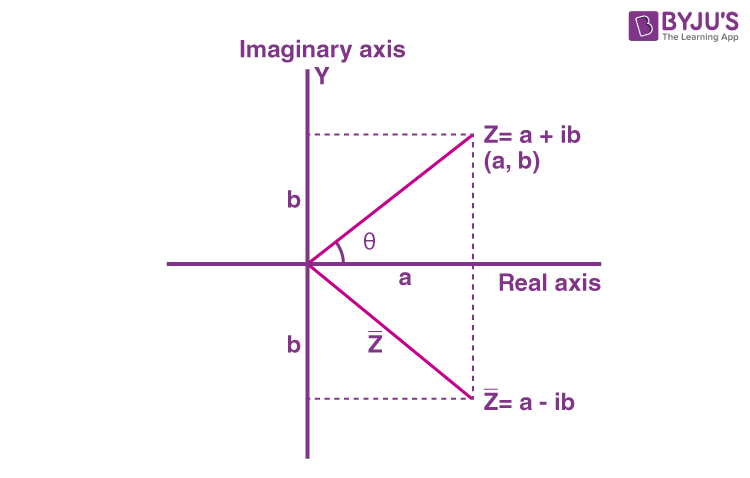
• The x-axis represents the real part.
• The y-axis represents the imaginary part.

3.3 Modulus and Argument

• The modulus (or absolute value) of a complex number is:

  $$|z| = \sqrt{a^2 + b^2}$$

• The argument $\theta$ is the angle from the positive real axis to the vector:

  $$\theta = \tan^{-1} \left( \frac{b}{a} \right), \quad \text{where } 0 \leq \theta < 2\pi$$

💡 Tip: For purely imaginary numbers (i.e., $a = 0$):

• If $b > 0$, then $\theta = \frac{\pi}{2}$
• If $b < 0$, then $\theta = \frac{3\pi}{2}$

3.4 Cartesian, Polar, and Exponential Forms

• Euler's Formula:

  $$\cos\theta + i\sin\theta = e^{i\theta}$$

• Cartesian Form:

  $$z = a + bi$$

• Polar Form:

  $$z = r(\cos\theta + i\sin\theta) = r\,\text{cis}\,\theta$$

• Exponential Form:

  $$z = r e^{i\theta}$$

  Where $r = |z|$ and $\theta = \arg(z)$

3.5 Operations in Polar/Exponential Form

Multiplication

• Multiply moduli and add arguments:

  $$z_1 z_2 = r_1 r_2 e^{i(\theta_1 + \theta_2)} = r_1 r_2\, \text{cis}(\theta_1 + \theta_2)$$

Division

• Divide moduli and subtract arguments:

  $$\frac{z_1}{z_2} = \frac{r_1}{r_2} e^{i(\theta_1 - \theta_2)} = \frac{r_1}{r_2}\, \text{cis}(\theta_1 - \theta_2)$$

3.6 De Moivre’s Theorem

• For powers of complex numbers:

  $$z^n = \left( r e^{i\theta} \right)^n = r^n e^{i n \theta}$$

• Using polar form:

  $$z^n = r^n (\cos n\theta + i\sin n\theta)$$

🔁 Multiply the argument by $n$ and raise the modulus to the $n^{\text{th}}$ power.

Reducing Large Arguments (Radian Mod)

• If the angle becomes too large, subtract $2\pi$ as many times as needed: $$\theta_{\text{reduced}} = \theta \mod 2\pi$$

3.7 Roots of Unity (Not in Exam)

• The $n^{\text{th}}$ roots of 1 are:

  $$z_k = \cos\left( \frac{2\pi k}{n} \right) + i\sin\left( \frac{2\pi k}{n} \right), \quad \text{for } k = 0, 1, \dots, n-1$$

• Example for $z^3 = 1$:

  • $z_1 = \cos(0) + i\sin(0) = 1$
  • $z_2 = \cos\left( \frac{2\pi}{3} \right) + i\sin\left( \frac{2\pi}{3} \right)$
  • $z_3 = \cos\left( \frac{4\pi}{3} \right) + i\sin\left( \frac{4\pi}{3} \right)$

---

4. Related Rates, Differentials, and Newton’s Method

4.1 Related Rates & Chain Rule

Related Rates

• If $y = f(x)$, the rate of change of $y$ with respect to $x$ is defined as:

  $$\frac{dy}{dx} = f'(x)$$

• $\frac{dy}{dx}$ is Leibniz's notation for the derivative, and it represents the rate at which $y$ changes with $x$.

Chain Rule

• If $y = f(x)$ and $x = f(t)$, then:

  $$\frac{dy}{dt} = \frac{dy}{dx} \cdot \frac{dx}{dt}$$

• This rule connects rates of change between dependent variables.

Key Ideas for Solving Related Rates Problems

• Use the chain rule to relate changing quantities.
• Establish an equation that relates all variables.
• Differentiate both sides with respect to time.
• Ratios often appear and can simplify or cancel out variables.

4.2 Differentials & Linear Approximation

Differentials

• Given $y = f(x)$:

  $$\frac{dy}{dx} = f'(x) \quad \Rightarrow \quad dy = f'(x)\,dx$$

• Differentials are used to estimate small changes in $y$ based on small changes in $x$.

• Used for approximation:

  $$dy \approx f'(x_1)(x_2 - x_1)$$

  Where $dy$ approximates $f(x_2) - f(x_1)$.

Linear Approximation

• The linear approximation formula at $x = a$ is:

  $$L(x) = f(a) + f'(a)(x - a)$$

• This estimates $f(x)$ using a tangent line near $x = a$.

4.3 Newton’s Method

• An iterative method for approximating roots of a function.

• Formula:

  $$x_{n+1} = x_n - \frac{f(x_n)}{f'(x_n)}$$

• Process:

  1. Start with an initial guess $x_0$
  2. Use the formula to compute better approximations
  3. Repeat until convergence

• Works well when:

  • $f(x)$ is differentiable near the root
  • $f'(x)$ is not zero near the root

---

5. Inverse & Transcendental Functions

5.1 Inverse Functions

Definition

• A function $f$ has an inverse $f^{-1}$ if it is one-to-one.

• The graph of $f^{-1}(x)$ is the reflection of $f(x)$ about the line $y = x$.

• Point relationship:

  $$\text{If } f(a) = b, \text{ then } f^{-1}(b) = a$$ $$(x = a, y = b) \iff (x = b, y = a)$$

Inverse Function Theorem

• If $f(b) = a$, then:

  $$(f^{-1})'(a) = \frac{1}{f'(b)}$$

5.2 Exponential Functions

Laws of Exponents

• $$a^{x+y} = a^x \cdot a^y$$
• $$a^{x-y} = \frac{a^x}{a^y}$$
• $$(a^x)^y = a^{xy}$$
• $$(ab)^x = a^x b^x$$

Derivative

• $$\frac{d}{dx}(e^x) = e^x$$
• $$\frac{d}{dx}(e^{f(x)}) = e^{f(x)} \cdot f'(x)$$

Integral

• $$\int e^x dx = e^x + C$$
• $$\int e^{f(x)} dx = \frac{e^{f(x)}}{f'(x)} + C$$

5.3 Logarithmic Functions

Laws of Logarithms

• $$\log_e(xy) = \log_e x + \log_e y$$
• $$\log_e\left(\frac{x}{y}\right) = \log_e x - \log_e y$$
• $$\log_e(x^r) = r \log_e x$$

⚠️ Note: $(\log_e x)^r \neq r \log_e x$

Derivative

• $$\frac{d}{dx} \ln x = \frac{1}{x}$$
• $$\frac{d}{dx} \ln(f(x)) = \frac{f'(x)}{f(x)}$$

Integral

• $$\int \frac{1}{x} dx = \ln|x| + C$$
• $$\int \frac{f'(x)}{f(x)} dx = \ln|f(x)| + C$$

5.4 Inverse Trigonometric Functions

Inverse Sine

• $$\frac{d}{dx}(\sin^{-1}x) = \frac{1}{\sqrt{1 - x^2}}$$
• $$\int \frac{1}{\sqrt{1 - x^2}} dx = \sin^{-1}(x) + C$$

Inverse Cosine

• $$\frac{d}{dx}(\cos^{-1}x) = -\frac{1}{\sqrt{1 - x^2}}$$

Inverse Tangent

• $$\frac{d}{dx}(\tan^{-1}x) = \frac{1}{1 + x^2}$$
• $$\int \frac{1}{1 + x^2} dx = \tan^{-1}(x) + C$$

Solving Using Triangle

• Use a triangle to define angle relationships.
• Use geometry to rewrite expressions in simpler terms.

5.5 Hyperbolic Functions

Definition of Hyperbolic Functions

• $$\sinh x = \frac{e^x - e^{-x}}{2}$$
• $$\cosh x = \frac{e^x + e^{-x}}{2}$$
• $$\tanh x = \frac{\sinh x}{\cosh x} = \frac{e^x - e^{-x}}{e^x + e^{-x}}$$
• $$\csch x = \frac{1}{\sinh x}, \quad \sech x = \frac{1}{\cosh x}, \quad \coth x = \frac{\cosh x}{\sinh x}$$

💡 $\sinh(\log(e^x)) = \frac{e^x - e^{-x}}{2}$
Think of $e^x$ as a variable — so you can still use $\sinh$ even if it’s not explicitly written as $e^x$

Hyperbolic Identities

• $$\sinh(-x) = -\sinh x, \quad \cosh(-x) = \cosh x$$
• $$\cosh^2 x - \sinh^2 x = 1$$
• $$1 - \tanh^2 x = \sech^2 x$$
• $$\sinh(x + y) = \sinh x \cosh y + \cosh x \sinh y$$
• $$\cosh(x + y) = \cosh x \cosh y + \sinh x \sinh y$$
• $$\tanh(x + y) = \frac{\tanh x + \tanh y}{1 + \tanh x \tanh y}$$
• $$\tanh(x - y) = \frac{\tanh x - \tanh y}{1 - \tanh x \tanh y}$$

Derivatives of Hyperbolic Functions

• $$\frac{d}{dx} \sinh x = \cosh x$$
• $$\frac{d}{dx} \cosh x = \sinh x$$
• $$\frac{d}{dx} \tanh x = \sech^2 x$$
• $$\frac{d}{dx} \coth x = -\csch^2 x$$
• $$\frac{d}{dx} \sech x = -\sech x \tanh x$$
• $$\frac{d}{dx} \csch x = -\csch x \coth x$$

Integrals of Hyperbolic Functions

• $$\int \sinh x \, dx = \cosh x + C$$
• $$\int \cosh x \, dx = \sinh x + C$$
• $$\int \sech^2 x \, dx = \tanh x + C$$
• $$\int \csch^2 x \, dx = -\coth x + C$$
• $$\int \sech x \tanh x \, dx = -\sech x + C$$
• $$\int \csch x \coth x \, dx = -\csch x + C$$

Inverse Hyperbolic Functions

• $$\sinh^{-1} x = \ln \left( x + \sqrt{x^2 + 1} \right), \quad x \in \mathbb{R}$$
• $$\cosh^{-1} x = \ln \left( x + \sqrt{x^2 - 1} \right), \quad x \ge 1$$
• $$\tanh^{-1} x = \frac{1}{2} \ln \left( \frac{1 + x}{1 - x} \right), \quad -1 < x < 1$$
• $$\coth^{-1} x = \frac{1}{2} \ln \left( \frac{x + 1}{x - 1} \right), \quad |x| > 1$$
• $$\sech^{-1} x = \ln \left( \frac{1 + \sqrt{1 - x^2}}{x} \right), \quad 0 < x \le 1$$
• $$\csch^{-1} x = \ln \left( \frac{1}{x} + \frac{\sqrt{1 + x^2}}{|x|} \right), \quad x \ne 0$$

Derivatives of Inverse Hyperbolic Functions

• $$\frac{d}{dx} \sinh^{-1} x = \frac{1}{\sqrt{1 + x^2}}$$
• $$\frac{d}{dx} \cosh^{-1} x = \frac{1}{\sqrt{x^2 - 1}}$$
• $$\frac{d}{dx} \tanh^{-1} x = \frac{1}{1 - x^2}$$
• $$\frac{d}{dx} \coth^{-1} x = \frac{1}{1 - x^2}$$
• $$\frac{d}{dx} \sech^{-1} x = \frac{-1}{x \sqrt{1 - x^2}}$$
• $$\frac{d}{dx} \csch^{-1} x = \frac{-1}{|x| \sqrt{1 + x^2}}$$

---

6. Techniques of Integration

6.1 Integration by Substitution

• Observe the function and choose an expression to substitute as $u$

  • The chosen part should be easily differentiable and cancel with the remaining part of the integrand.

• When $u = g(x)$, we differentiate:

  $$\frac{du}{dx} = g'(x) \quad \Rightarrow \quad dx = \frac{du}{g'(x)}$$

• Replace $dx$ and the corresponding expression in the integrand with $du$ and $u$.

• For definite integrals, convert limits of $x$ into limits in terms of $u$:

  $$\int_a^b f(g(x))g'(x)\ dx = \int_{u(a)}^{u(b)} f(u)\ du$$

6.2 Integration by Parts

• Formula:

  $$\int u\frac{dv}{dx}\ dx = uv - \int \frac{du}{dx}v\ dx \quad \iff \quad \int u\ dv = uv - \int v\ du$$

• Use the LIATE Rule to decide which part of the integrand should be $u$:

  • $L$: Logarithmic functions ($\ln x$)
  • $I$: Inverse trigonometric functions ($\sin^{-1}x$, $\tan^{-1}x$, ...)
  • $A$: Algebraic functions ($x$, $x^2$, $x^n$)
  • $T$: Trigonometric functions ($\sin x$, $\cos x$, ...)
  • $E$: Exponential functions ($e^x$)

⚠️ The LIATE rule is a guideline, not a strict rule — exceptions may apply depending on the problem.

Integration by Parts for Inverse Trig Functions

• When integrating an inverse trigonometric function (like $\tan^{-1}x$), use the trick:

  $$\int \tan^{-1}x\ dx = \int \tan^{-1}x \cdot 1\ dx$$

• Then apply integration by parts with:

  • $u = \tan^{-1}x$
  • $dv = dx$

6.3 Integration by Partial Fractions

• Use algebra to decompose a rational function into simpler fractions that are easier to integrate.

Case 1: Two linear factors

• For an expression like:

  $$\frac{px + q}{(ax + b)(cx + d)} = \frac{A}{ax + b} + \frac{B}{cx + d}$$

Case 2: Repeated linear factors

• For a repeated linear factor like $(ax + b)^2$:

  $$\frac{px + q}{(ax + b)^2(cx + d)} = \frac{A}{ax + b} + \frac{B}{(ax + b)^2} + \frac{C}{cx + d}$$

• For $(ax + b)^n$, general form:

  $$\frac{P(x)}{(ax + b)^n} = \frac{A_1}{ax + b} + \frac{A_2}{(ax + b)^2} + \cdots + \frac{A_n}{(ax + b)^n}$$

Case 3: Linear and Irreducible Quadratic

• If the denominator has both a linear factor and a non-factorizable quadratic $(cx^2 + d)$:

  $$\frac{px + q}{(ax + b)(cx^2 + d)} = \frac{A}{ax + b} + \frac{Bx + C}{cx^2 + d}$$

• After decomposition, integrate each term using basic rules or known formulas.

---

7. Definite Integrals & Numerical Integration

7.1 The Definite Integral

• A definite integral is evaluated over a specific interval:

  $$\int_a^b f(x)\ dx = [F(x)]_a^b = F(b) - F(a)$$

Substitution with Limits

• When using substitution in definite integrals:

  $$u = f(x), \quad \frac{du}{dx} = f'(x) \quad \Rightarrow \quad dx = \frac{du}{f'(x)}$$

• Convert limits:

  $$\int_{x_1}^{x_2} f(x)\ dx = \int_{u_1 = f(x_1)}^{u_2 = f(x_2)} \frac{u}{f'(x)}\ du$$

Integration by Parts with Limits

• Formula with limits applied:

  $$\int_a^b u \frac{dv}{dx}\ dx = [uv]_a^b - \int_a^b \frac{du}{dx}v\ dx$$

7.2 The Trapezoidal Rule

• Approximate the area under a curve by dividing it into trapezoids:

  $$\int_a^b f(x)\ dx \approx \frac{h}{2} \left[ y_0 + y_n + 2(y_1 + y_2 + \cdots + y_{n-1}) \right]$$

• Step size (height of each trapezoid):

  $$h = \frac{b - a}{n}$$

• Nodes:

  $$x_0 = a,\ x_1 = a + h,\ \ldots,\ x_n = b$$

• Make a table of $x$ and corresponding $y = f(x)$ values to compute.

7.3 Simpson’s Rule

• More accurate than the trapezoidal rule, uses parabolas:

  $$\int_a^b f(x)\ dx \approx \frac{h}{3} \left[ y_0 + y_n + 4(y_1 + y_3 + \cdots + y_{n-1}) + 2(y_2 + y_4 + \cdots + y_{n-2}) \right]$$

• Equivalent in simple terms:

  $$\int_a^b f(x)\ dx \approx \frac{h}{3} \left[ \text{First + Last} + 4(\text{Odds}) + 2(\text{Evens}) \right]$$

• Step size:

  $$h = \frac{b - a}{n}, \quad \text{where $n$ is even}$$

• Make a table of $x_i$ and $y_i = f(x_i)$ values to compute.

7.4 Trapezoidal vs Simpson’s Rule

• Trapezoidal Rule approximates area using straight lines (trapezoids).
• Simpson’s Rule approximates area using quadratic curves (parabolas).
• Simpson’s Rule is usually more accurate if $f(x)$ is smooth and $n$ is even.

---

8. First-Order Linear Differential Equations

8.1 Introduction to Differential Equations

• A differential equation is an equation involving a function and its derivatives.

Order of a Differential Equation

• Determined by the highest derivative in the equation:

  $$\frac{dy}{dx} \Rightarrow \text{1st order}, \quad \frac{d^2y}{dx^2} \Rightarrow \text{2nd order}, \quad \frac{d^n y}{dx^n} \Rightarrow \text{n-th order}$$

Degree of a Differential Equation

• The degree is the exponent of the highest order derivative (if the equation is polynomial in derivatives):

  $$\left( \frac{dy}{dx} \right)^2 \Rightarrow \text{1st order, 2nd degree}, \quad \left( \frac{d^4 y}{dx^4} \right)^1 \Rightarrow \text{4th order, 1st degree}$$

Linear vs Nonlinear Differential Equations

• A differential equation is linear if:
  • All $y$ terms and derivatives are of degree 1
  • Derivatives of $y$ are not multiplied by each other

8.2 Standard Form

• A first-order linear differential equation is written as:

  $$\frac{dy}{dx} + P(x)y = Q(x)$$

• If $Q(x) = 0$, the equation is homogeneous.

• If $Q(x) \ne 0$, the equation is non-homogeneous.

8.3 The Method of Separation of Variables

General Method

• Rearrange to separate $x$ and $y$:

  $$f(y)\frac{dy}{dx} = g(x)$$

• Integrate both sides:

  $$\int f(y) \frac{dy}{dx} dx = \int g(x)\ dx$$ $$\Rightarrow \int f(y)\ dy = \int g(x)\ dx$$

• General solution:

  $$F(y) = G(x) + C$$

• If initial values are given, substitute to find $C$ for the particular solution.

Applications

Population Growth and Decay

• General model:

  $$P(t) = P_0 e^{kt}$$

Newton’s Law of Cooling

• Temperature model:

  $$T(t) = P + T_0 e^{kt}$$

8.4 Integrating Factors

General Form

• Arrange into standard linear form:

  $$\frac{dy}{dx} + p(x)y = Q(x)$$

Step 1: Find Integrating Factor

• The integrating factor is:

  $$v(x) = e^{\int p(x)\ dx}$$

• Derivative of $v(x)$:

  $$v'(x) = v(x)p(x)$$

Step 2: Multiply Equation by Integrating Factor

• Multiply both sides by $v(x)$:

  $$v(x) \frac{dy}{dx} + v(x)p(x)y = v(x)Q(x)$$

• Recognize the left side as the derivative of a product:

  $$\frac{d}{dx} [v(x)y] = v(x)Q(x)$$

Step 3: Integrate Both Sides

• Integrate:

  $$v(x)y = \int v(x)Q(x)\ dx + C$$

• Solve for $y$:

  $$y = \frac{1}{v(x)} \left( \int v(x)Q(x)\ dx + C \right)$$

• If initial condition is given, substitute to find $C$.

8.5 When to Use Which Method?

• Given:

  $$\frac{dy}{dx} + p(x)y = q(x)$$

• If $q(x) = 0$: homogeneous → use separation of variables.

• If $q(x) \ne 0$: non-homogeneous → use integrating factors (separation won't work).

---

9. Second-Order Differential Equations

9.1 Standard Form

• A second-order linear differential equation has the form:

  $$P(x)y'' + Q(x)y' + R(x)y = f(x)$$

• For constant coefficients, this becomes:

  $$ay'' + by' + cy = f(x)$$

• If $f(x) = 0$, the equation is homogeneous.

• If $f(x) \ne 0$, the equation is non-homogeneous.

9.2 Characteristic Equation and General Solution

• Standard homogeneous form:

  $$ay'' + by' + cy = 0$$

• Associated characteristic equation:

  $$am^2 + bm + c = 0$$

• Solve for roots $m_1$ and $m_2$ (via quadratic formula, factoring, etc.)

• General solution depends on the type of roots:

Case 1: Real and Distinct Roots ($m_1 \ne m_2$)

• Solution:

  $$y(t) = c_1 e^{m_1 t} + c_2 e^{m_2 t}$$

Case 2: Real and Equal Roots ($m_1 = m_2$)

• Solution:

  $$y(t) = (c_1 + c_2 t)e^{m_1 t}$$

Case 3: Complex Roots ($m = p \pm qi$)

• Solution:

  $$y(t) = e^{pt}(c_1 \cos qt + c_2 \sin qt)$$

• Use initial conditions to solve for constants $c_1$, $c_2$ if provided.

9.3 Spring-Mass System

No Friction

• Forces:

  $$\begin{cases} F = ma \Rightarrow F = mx'' \\ F_s = -kx \end{cases}$$

• Resulting DE:

  $$mx'' + kx = 0 \Rightarrow x'' + \omega^2 x = 0, \quad \omega^2 = \frac{k}{m}$$

• Characteristic equation:

  $$m^2 + \omega^2 = 0 \Rightarrow m = \pm i\omega$$

• General solution:

  $$x(t) = c_1 \cos \omega t + c_2 \sin \omega t$$

With Friction

• Additional force: damping force $F_D = -cv$

• Forces:

  $$\begin{cases} F = ma \Rightarrow F = mx'' \\ F_s = -kx \\ F_D = -cx' \end{cases}$$

• Resulting DE:

  $$mx'' + cx' + kx = 0$$

• Characteristic equation:

  $$mr^2 + cr + k = 0$$

• Roots:

  $$r = \frac{-c \pm \sqrt{c^2 - 4km}}{2m}$$

Types of Motion Based on Roots

Overdamped Motion ($c^2 > 4km$)

• Roots are real and distinct: $r_1 < 0$, $r_2 < 0$

  $$x(t) = c_1 e^{r_1 t} + c_2 e^{r_2 t}$$

Critically Damped Motion ($c^2 = 4km$)

• Roots are real and equal: $r_1 = r_2 < 0$

  $$x(t) = (c_1 + c_2 t)e^{r_1 t}$$

Underdamped Motion ($c^2 < 4km$)

• Roots are complex: $r = p \pm qi$ with $p < 0$

  $$x(t) = e^{pt}(c_1 \cos qt + c_2 \sin qt)$$

---

10. Non-Homogeneous Second-Order Linear Differential Equations

10.1 Standard Form

• General form of the equation:

  $$ax'' + bx' + cx = f(t)$$

• If $f(t) = 0$, it's homogeneous.

• If $f(t) \ne 0$, it's non-homogeneous.

10.2 Solution Steps

1. Find the Complementary Solution $x_c$ by solving the homogeneous equation:

   $$ax'' + bx' + cx = 0$$
   • Solve for roots using the characteristic equation.
   • Refer to: [[Solutions of Second-Order DEs]].

2. Find a Particular Solution $x_p$ of the non-homogeneous equation.

3. Combine the Solutions:

   $$x(t) = x_c + x_p$$

10.3 The Method of Undetermined Coefficients

We focus on:

• $f(t) = k\cos(bt)$
• $f(t) = k\sin(bt)$
• $f(t) = k\cos(bt) + l\sin(bt)$

First Method

1. Assume:

   $$x_p = A\cos(bt) + B\sin(bt)$$

2. Compute derivatives $x_p'$ and $x_p''$.

3. Substitute into:

   $$ax''_p + bx'_p + cx_p = f(t)$$

4. Match coefficients of $\cos(bt)$ and $\sin(bt)$ on both sides to find $A$ and $B$.

Second Method (if First Fails)

Use if:

$$ax''_p + bx'_p + cx_p = 0 \text{ when substituted into } f(t) \ne 0$$

1. Assume:

   $$x_p = At\cos(bt) + Bt\sin(bt)$$

2. Compute $x_p'$ and $x_p''$ using product rule.

3. Substitute into equation and solve for $A$, $B$.

Note:

• Try First Method first.
• If it fails, use the Second Method.

10.4 Forced Oscillations

• Focus: solving DEs with oscillating forcing function.

General Form

$$x'' + \omega^2 x = a\sin(bt), \quad x(0) = 0,\quad x'(0) = 0$$

• Mass starts at rest and equilibrium.

Three Cases

1. Case 1: $\omega \ne b$ (Periodic Motion)
   Use:

   $$x_p = A\cos(bt) + B\sin(bt)$$

2. Case 2: $\omega = b$ (Resonance)
   Use:

   $$x_p = At\cos(bt) + Bt\sin(bt)$$

3. Case 3: $\omega \approx b$ (Beat)
   Use same form as Case 1, but will produce beat phenomenon.

General Solution

$$x(t) = x_c + x_p$$

• Use initial conditions to solve for constants $c_1$, $c_2$.

10.5 Beat Behavior

• Equation:

  $$x'' + \omega^2 x = a \sin(bt)$$

• If $\omega \approx b$, the system exhibits beats — the amplitude varies slowly over time.

---

11. Sequences & Series

11.1 Introduction to Infinite Sequences and Series

Geometric Sequences

• The general form of a geometric sequence:

  $$a,\ ar,\ ar^2,\ ar^3,\ \dots,\ ar^n,\ \dots$$
  • $a$ is the first term
  • $r$ is the common ratio

Geometric Series

• An infinite geometric series is written as:

  $$\sum^{\infty}_{n=1} a_n = a_1 + a_2 + a_3 + \dots + a_n + \dots$$

• The n-th partial sum of the series is:

  $$S_n = a_1 + a_2 + a_3 + \dots + a_n = \sum^{n}_{k=1} a_k$$
  • Examples:
    • $S_1 = a_1$
    • $S_2 = a_1 + a_2$
    • $S_3 = a_1 + a_2 + a_3$
    • and so on...

Sum Formulas

• Sum to $n$ terms:

  $$S_n = \frac{a(1 - r^n)}{1 - r}, \quad r \ne 1$$

• Sum to infinity (when $|r| < 1$):

  $$S_\infty = \frac{a}{1 - r}$$

References

• LibreTexts – Geometric Sequences and Series
• YouTube: Geometric Series Explanation

---

11.2 The Ratio Test and Power Series

The Ratio Test

Given a series $\sum a_n$:

$$\lim_{n \to \infty} \left| \frac{a_{n+1}}{a_n} \right| = L$$

• If $L < 1$: the series converges
• If $L > 1$ or $L = \infty$: the series diverges
• If $L = 1$: the test is inconclusive

Example

Given:

$$a_n = \frac{2^n + 5}{3^n}$$

Then:

$$a_{n+1} = \frac{2^{n+1} + 5}{3^{n+1}}$$

Substitute into the ratio test formula.

Power Series

Power series form and convergence not elaborated here but related to the ratio test for determining convergence radius.

References

• YouTube: Factorial Pattern ((n-1)!)
• YouTube: Ratio Test Explanation