Mathematic 2 - Calculus 2 - Summary

1. Linear System

1.1 Linear Equations and Systems

• [[Linear "Equation and Systems" & Augmented Matrices]]

Linear Equation

• Variables like $x$, $y$, or $z$ must have power 1 and constant coefficients: $$a_1x_1+a_2x_2+\dots+a_nx_n = b \quad \text{or} \quad a_1x+a_2y+\dots+a_nz = b$$
• No variables multiplying each other.

Linear System and Its Solution

• System of equations: $$\begin{cases} a_1x_1+a_2x_2+\dots+a_nx_n = b_1 \\ a_{11}x_1+a_{12}x_2+\dots+a_{mn}x_n = b_2 \\ \vdots \\ a_{m1}x_1+a_{m2}x_2+\dots+a_{mn}x_n = b_m \end{cases}$$
• A solution satisfies all equations.
• Solutions:
  • No solution → parallel lines/planes
  • One solution → intersection point
  • Infinite solutions → equations are dependent

Augmented Matrices

Transform system into matrix of coefficients and constants:

$$\begin{cases} a_1x_1+a_2x_2+...+a_nx_n& =b_1 \\ a_{11}x_1+a_{12}x_2+...+a_{mn}x_n&=b_2 \\ & \Big\downarrow \\ a_{m1}x_1+a_{m2}x_2+...+a_{mn}x_n&=b_m \end{cases} \xrightarrow{\text{ Augmented Matrics }} \begin{pmatrix} a_1+a_2+...+a_n& =b_1 \\ a_{11}+a_{12}+...+a_{mn}&=b_2 \\ & \Big\downarrow \\ a_{m1}+a_{m2}+...+a_{mn}&=b_m \end{pmatrix}$$

1.2 Elementary Row Operations & Row-Reduced Matrices

• [[Elementary Row Operations & Row-Reduced Matrices]]

Elementary Row Operations

Used to simplify matrices for solving:

• Only operate by row (not by column).
• Matrix example: $$\begin{pmatrix} \color{violet}a & b & c & | & P \\ \color{violet}d & e & f & | & Q \\ \color{violet}g & h & i & | & R \end{pmatrix}$$

Three operations:

1. Multiply a row by a constant $$R_i \leftarrow kR_i$$
2. Swap two rows $$R_i \leftrightarrow R_j$$
3. Add a multiple of one row to another $$R_i \leftarrow R_i + kR_j$$

Row-Reduced Matrices

Transform into row-echelon or reduced row-echelon form:

• Final form (as system): $$\begin{cases} 1x + 0 + 0 = \Delta P \\ 0 + 1y + 0 = \Delta Q \\ 0 + 0 + 1z = \Delta R \end{cases}$$
• Final form (as matrix): $$\begin{pmatrix} 1 & 0 & 0 & | & \Delta P \\ 0 & 1 & 0 & | & \Delta Q \\ 0 & 0 & 1 & | & \Delta R \end{pmatrix}$$

Properties of Reduced Row-Echelon Form:

1. First nonzero element in each row is 1 (leading 1).
2. All-zero rows are at the bottom.
3. Each leading 1 is to the right of any leading 1 above it.
4. Each leading 1 is the only nonzero entry in its column.

• If only 1–3 are satisfied → row-echelon form
• If all 1–4 are satisfied → reduced row-echelon form

1.3 Gauss-Jordan Elimination

• [[Gauss-Jordan Elimination]]

Used to solve:

$$\begin{cases} ax + by + cz = P \\ dx + ey + fz = Q \\ gx + hy + iz = R \end{cases} \Rightarrow \begin{bmatrix} a & b & c & | & P \\ d & e & f & | & Q \\ g & h & i & | & R \end{bmatrix} \Rightarrow \begin{bmatrix} 1 & 0 & 0 & | & x \\ 0 & 1 & 0 & | & y \\ 0 & 0 & 1 & | & z \end{bmatrix}$$

Performing

• Change one row while keeping the others: $$\begin{bmatrix} a & b & c & | & P \\ d & e & f & | & Q \\ g & h & i & | & R \end{bmatrix} \xrightarrow{2R_1 - R_2} \begin{bmatrix} \Delta a & 0 & \Delta c & | & \Delta P \\ d & e & f & | & Q \\ g & h & i & | & R \end{bmatrix}$$

Then scale rows:

$$\begin{bmatrix} \Delta a & 0 & 0 & | & \Delta P \\ 0 & \Delta e & 0 & | & \Delta Q \\ 0 & 0 & \Delta i & | & \Delta R \end{bmatrix} \Rightarrow \text{multiply each by } \frac{1}{\Delta} \Rightarrow \begin{bmatrix} 1 & 0 & 0 & | & x \\ 0 & 1 & 0 & | & y \\ 0 & 0 & 1 & | & z \end{bmatrix}$$

Where:

• $x = \Delta P / \Delta a$
• $y = \Delta Q / \Delta e$
• $z = \Delta R / \Delta i$

Types of Solutions

• One solution: intersection point
  ![[Screenshot 2567-06-12 at 10.17.51.png|300]]
• Infinite solutions: same plane
  ![[Screenshot 2567-06-12 at 10.19.08.png|300]]
• No solution: $$\begin{pmatrix} 1 & 0 & 0 & | & 14 \\ 0 & 1 & -2 & | & 2 \\ 0 & 0 & 0 & | & 1 \end{pmatrix}$$

1.4 References

• https://www.youtube.com/watch?v=eYSASx8_nyg

---

2. Matrix Algebra

2.1 Matrices and Operations

• A matrix has $m$ rows and $n$ columns → its size is $m \times n$
• Column and Row matrices:
  • $n$ columns and 1 row: called a row vector
  • $m$ rows and 1 column: called a column vector

Square matrices

• If $m = n$, it is a square matrix

Diagonal matrices

• A square matrix where all off-diagonal entries are zero
• If the main diagonal has non-zero values, it is called a diagonal matrix

Zero matrices

• A matrix where all entries are 0

Identity matrices

• A diagonal matrix with all 1s on the diagonal
• Denoted by $I_n$

2.2 Operations of Matrices

Equality

• Two matrices are equal if they have the same size and corresponding entries are equal

Addition

• Add corresponding elements; both matrices must have the same size

Scalar Multiplication

• Multiply each entry of a matrix $A$ by a scalar $k$ to get $kA$

Matrix Multiplication

• Only valid if the number of columns of $A$ equals the number of rows of $B$
• Not commutative: $AB \ne BA$

Power of Square Matrix

• For integer $n \geq 0$:
  $A^0 = I$,
  $A^n = A \cdot A \cdot \ldots \cdot A$ (n times)

Transpose

• Switch rows with columns: $A^T$
• Tips:
  • Focus on the columns
  • When transposing powers: $(A^n)^T = (A^T)^n$

2.3 Properties of Matrix Operations

• $A + B = B + A$  (Commutative law of addition)
• $A + (B + C) = (A + B) + C$  (Associative law of addition)
• $A(BC) = (AB)C$  (Associative law of multiplication)
• $A(B + C) = AB + AC$  (Distributive law)
• $(B + C)A = BA + CA$  (Distributive law)
• $A + 0 = 0 + A = A$,  $A - A = 0$
• $0A = 0$,  $A0 = 0$
• $(A^T)^T = A$,  $(AB)^T = B^T A^T$

2.4 Matrix Inversion

Inverse Matrix

• Only square matrices have inverses
• For a matrix $A$, if $AA^{-1} = I$, then $A^{-1}$ is the inverse

Inverse of a $2 \times 2$ Matrix

If $ad - bc \ne 0$, then:

$$\begin{pmatrix} a & b \\ c & d \end{pmatrix}^{-1} = \frac{1}{ad - bc} \begin{pmatrix} d & -b \\ -c & a \end{pmatrix}$$

Finding Inverse using Gauss-Jordan

• Augment matrix $A$ with identity matrix $I_n$:
  $A \, | \, I_n \longrightarrow I_n \, | \, A^{-1}$

2.5 Solving Linear System using Inverse

• For a system $AX = B$, solve as:
  $AX = B \Rightarrow (A^{-1}A)X = A^{-1}B \Rightarrow IX = A^{-1}B \Rightarrow \color{tomato}{X = A^{-1}B}$

• Visual reference:

$$\begin{aligned} &\left\{ \begin{array}{cccccc} a_{11}x_1 & + a_{12}x_2 & + \cdots & + a_{1n}x_n &= b_1 \\ a_{21}x_1 & + a_{22}x_2 & + \cdots & + a_{2n}x_n &= b_2 \\ \vdots & \vdots & & \vdots & \vdots \\ a_{m1}x_1 & + a_{m2}x_2 & + \cdots & + a_{mn}x_n &= b_m \\ \end{array} \right. \\[1em] \Rightarrow\quad &\left( \begin{array}{cccc} a_{11}x_1 & + a_{12}x_2 & + \cdots & + a_{1n}x_n \\ a_{21}x_1 & + a_{22}x_2 & + \cdots & + a_{2n}x_n \\ \vdots & \vdots & & \vdots \\ a_{m1}x_1 & + a_{m2}x_2 & + \cdots & + a_{mn}x_n \\ \end{array} \right) = \left( \begin{array}{c} b_1 \\ b_2 \\ \vdots \\ b_m \\ \end{array} \right) \\[1em] \Rightarrow\quad &\left( \begin{array}{cccc} a_{11} & a_{12} & \cdots & a_{1n} \\ a_{21} & a_{22} & \cdots & a_{2n} \\ \vdots & \vdots & & \vdots \\ a_{m1} & a_{m2} & \cdots & a_{mn} \\ \end{array} \right) \left( \begin{array}{c} x_1 \\ x_2 \\ \vdots \\ x_n \\ \end{array} \right) = \left( \begin{array}{c} b_1 \\ b_2 \\ \vdots \\ b_m \\ \end{array} \right) \end{aligned}$$

---

3. Determinants

3.1 Determinants by Cofactor Expansion

• 2x2 Determinant for Inverse Matrix
  If

  $$A = \begin{pmatrix} a & b \\ c & d \end{pmatrix}, \quad A^{-1} = \frac{1}{ad - bc} \begin{pmatrix} d & -b \\ -c & a \end{pmatrix}$$

• Determinant of $n \times n$ Matrix:

  • Use Minor, Cofactor, and optionally Cross Product
  • Minor $M_{ij}$ is the matrix that results from removing the $i$th row and $j$th column
  • Cofactor $C_{ij} = (-1)^{i+j} M_{ij}$
  • Trick:
    • You can perform cofactor expansion along any row or column
    • Use row/column with the most zeros to simplify
    • For 3×3 matrix: $$|A| = a_{11}C_{11} + a_{12}C_{12} + a_{13}C_{13}$$

3.2 Determinants by Row and Column Reduction

• Triangular Matrices (Upper/Lower/Diagonal):

  • Determinant is product of diagonal: $$|A| = a_{11} a_{22} \cdots a_{nn}$$

• Elementary Row/Column Operations:

  • Row swap ($R_i \leftrightarrow R_j$) → sign change
  • Multiply row by scalar → determinant multiplied
  • Safe operation: $R_i \leftarrow R_i + kR_j$ (no change in determinant)

3.3 Cramer's Rule

• Solve $AX = B$ using determinants: $$x_i = \frac{|A_i|}{|A|}, \quad \text{where } A_i \text{ is A with column } i \text{ replaced by } B$$
• Effective only for small systems (2×2 or 3×3)
• For $n = 2$ and $n = 3$, substitute column-wise and solve using determinant rules

3.4 Volume of a Tetrahedron

• Given vertices $(x_1, y_1, z_1), \dots, (x_4, y_4, z_4)$: $$V = \pm \frac{1}{6} \begin{vmatrix} x_1 & y_1 & z_1 & 1 \\ x_2 & y_2 & z_2 & 1 \\ x_3 & y_3 & z_3 & 1 \\ x_4 & y_4 & z_4 & 1 \end{vmatrix}$$
• Always take the positive value of the result as volume

---

4 - Functions of Several Variables 1

4.1 Introduction, Domains, and Graphs

Domain and Range

• Check for square roots, denominators, or other conditions that could lead to undefined expressions.
• To find the range, observe the min/max values the expression can take.

4.2 Level Curves and Contour Maps

Level Curves

• Level curves are the 2D projections (bird’s-eye view) of surfaces where $z = f(x, y)$ is constant.
• Set $z = k$ (where $k$ is a constant) and solve for the relation between $x$ and $y$.

Contour Maps

• A contour map consists of multiple level curves at different heights $z = a, b, c, \dots$.
• Each curve corresponds to the same function value, representing height.

References:

• Video 1
• Video 2

4.3 Partial Derivatives

Concept

• For $f(x,y)$:
  • $$\frac{\partial f}{\partial x} \Rightarrow \text{treat } y \text{ as constant}$$
  • $$\frac{\partial f}{\partial y} \Rightarrow \text{treat } x \text{ as constant}$$
• For $f(x, y, z)$: hold two variables constant while differentiating with respect to the third.

Geometrical Interpretation

• $\displaystyle\frac{\partial f}{\partial x}$: change in $z = f(x, y)$ in the $x$-direction while $y$ is fixed
• $\displaystyle\frac{\partial f}{\partial y}$: change in $z = f(x, y)$ in the $y$-direction while $x$ is fixed

References:

• Geometric Interpretation

4.4 Chain Rules

Case 1: Simple Parametric Chain Rule

If $z = f(x, y)$ and $x = g(t), y = h(t)$:

$$\frac{dz}{dt} = \frac{\partial z}{\partial x}\frac{dx}{dt} + \frac{\partial z}{\partial y}\frac{dy}{dt}$$

Case 2: Multivariable Parametric Chain Rule

If $z = f(x, y)$ and $x = g(s, t), y = h(s, t)$:

• $$\frac{\partial z}{\partial s} = \frac{\partial z}{\partial x}\frac{\partial x}{\partial s} + \frac{\partial z}{\partial y}\frac{\partial y}{\partial s}$$
• $$\frac{\partial z}{\partial t} = \frac{\partial z}{\partial x}\frac{\partial x}{\partial t} + \frac{\partial z}{\partial y}\frac{\partial y}{\partial t}$$

• $s, t$ are independent variables

• $x, y$ are intermediate variables

• $z$ is the dependent variable

General Chain Rule for Many Variables

Let $w = f(x, y, z, t, \dots)$:

• $$\frac{\partial w}{\partial u} = \frac{\partial w}{\partial x}\frac{\partial x}{\partial u} + \frac{\partial w}{\partial y}\frac{\partial y}{\partial u} + \frac{\partial w}{\partial z}\frac{\partial z}{\partial u} + \frac{\partial w}{\partial t}\frac{\partial t}{\partial u} + \dots$$
• $$\frac{\partial w}{\partial v} = \frac{\partial w}{\partial x}\frac{\partial x}{\partial v} + \frac{\partial w}{\partial y}\frac{\partial y}{\partial v} + \frac{\partial w}{\partial z}\frac{\partial z}{\partial v} + \frac{\partial w}{\partial t}\frac{\partial t}{\partial v} + \dots$$

• Extend for more independent variables as needed.

---

5. Functions of Several Variables 2

5.1 Directional Derivatives

Concept

• Directional derivative:
  $D_{\vec{u}}f(x_0, y_0)$ denotes the directional derivative of $f$ at $(x_0, y_0)$ in the direction of unit vector $\vec{u}$.
• Partial derivatives consider only one direction (x or y), but the directional derivative considers any direction:

$$D_{\vec{u}}f(x, y) = \nabla f(x, y) \cdot \vec{u} = \color{tomato} f_x(x, y) \cdot a + f_y(x, y) \cdot b$$

Unit Vector

• Given vector $v$: $$\vec{u} = \frac{v}{|v|} = \langle a, b \rangle$$
• Given an angle $\theta$ with the x-axis:
  • $a = \cos \theta$, $b = \sin \theta$
  • Since $|\vec{u}| = 1$, $\vec{u} = \langle \cos \theta, \sin \theta \rangle$

5.2 Gradient Vector

Gradient Definition

• The gradient vector $\nabla f(x, y, z)$ is:

$$\nabla f(x, y, z) = \left\langle f_x, f_y, f_z \right\rangle = \frac{\partial f}{\partial x} \, \mathbf{i} + \frac{\partial f}{\partial y} \, \mathbf{j} + \frac{\partial f}{\partial z} \, \mathbf{k}$$

• It is the vector sum of all partial derivatives, pointing in the direction of steepest increase.

5.3 Tangent Planes

Equation of Plane

• Let $p(x_0, y_0, z_0)$ be the point of tangency.
• General form (based on gradient and point):

$$z = a(x - x_0) + b(y - y_0) + z_0$$

• Since $a = f_x(x_0, y_0)$ and $b = f_y(x_0, y_0)$:

$$\color{tomato} P(x, y) = f_x(x_0, y_0)(x - x_0) + f_y(x_0, y_0)(y - y_0) + f(x_0, y_0)$$

Derivative with Respect to Each Variable

• Let $P(x, y)$ be the tangent plane function.

• Partial with respect to $x$:

$$P_x(x, y) = a \quad \Rightarrow \quad P_x(x_0, y_0) = a = \color{tomato} f_x(x_0, y_0)$$

• Partial with respect to $y$:

$$P_y(x, y) = b \quad \Rightarrow \quad P_y(x_0, y_0) = b = \color{tomato} f_y(x_0, y_0)$$

5.4 Analogy to 1D Tangent Lines

• For 1D function $f(x)$:

$$\begin{cases} L(x_0) = f(x_0) \\ L'(x_0) = f'(x_0) \end{cases}$$

• For 2D surface $f(x, y)$ and tangent plane $P(x, y)$:

$$\begin{cases} P(x_0, y_0) = f(x_0, y_0) \\ \begin{cases} P_x(x_0, y_0) = f_x(x_0, y_0) \\ P_y(x_0, y_0) = f_y(x_0, y_0) \end{cases} \end{cases}$$

References

• YouTube: Directional Derivatives & Tangent Planes

---

Week 6 - Double Integrals 1

6.1 Double Integrals over General Regions

Concept

• When the shape is not a rectangle, use directional slicing (horizontal or vertical).
• If two bounding curves are given, find the intercept points between them first to determine the limits of integration.
• Points of intersection will define:
  • $x$-range: $x \in [a, b]$
  • $y$-range: $y \in [c, d]$

Choosing the Order of Integration

• You may integrate with respect to $y$ first or $x$ first — choose the easier way.

Example:

• Respect to $y$ (vertical strips):

  $$\int_a^b \int_{x^2}^{2x} f(x, y) \, dy \, dx$$

• Respect to $x$ (horizontal strips):

  $$\int_c^d \int_{y/2}^{\sqrt{y}} f(x, y) \, dx \, dy$$

General Form (Vertical Strip):

• If integrating in $y$ direction, use: $$V = \int_a^b \int_{g_1(x)}^{g_2(x)} f(x, y) \, dy \, dx$$

General Form (Horizontal Strip):

• If integrating in $x$ direction, use: $$V = \int_c^d \int_{h_1(y)}^{h_2(y)} f(x, y) \, dx \, dy$$

References

• YouTube: Double Integrals General Region

6.2 Reversing the Order of Integration

Concept

• Used when the current order of integration is hard to compute.
• Unlike double integrals over rectangles (with constant bounds), these often have variable bounds.
• You can switch from $dy \to dx$ or vice versa, depending on the region.

Strip Visualization

• Vertical Strip (dy first): fix $x$, integrate over $y$
• Horizontal Strip (dx first): fix $y$, integrate over $x$

Rewriting Limits

• Given:

  $$\int_c^d \int_{g(x)}^b f(x, y) \, dy \, dx$$

• First analyze the bounds:

  • $x \in [c, d]$
  • $y \in [g(x), b]$

• Sketch the region: include $x = c$, $x = d$, $y = g(x)$, and $y = b$.

• Then reverse the order:

  $$\int_m^l \int_k^{h(y)} f(x, y) \, dx \, dy$$
  • New bounds are derived from the region in the graph.

References

• YouTube (Explained Clearly)
• Short Example

---

Mathematic 2 - Statistic - Summary

1. Introduction to Statistics

1.1 Introduction to Statistics & Classification of Data

Concept

• Definition of statistical methods:

  • Population: Statistic from the whole population (not practical).
    • Parameter: Summarizes data from a population.
  • Sample: Statistic from a subset (more feasible).
    • Statistic: Summarizes data from a sample.
  • Simple random sample: Considers all people equally.

• Accuracy check for sample:

  $$|\text{sample average} - \text{population average}| \leq n$$
  • Big difference: inaccurate
  • Small difference: accurate

• Confidence interval: Interval where the true value is likely to lie.

Types of Data

• Qualitative Nominal: Categorical, no order (e.g., Gender, State).
• Qualitative Ordinal: Categorical with order (e.g., Grades, Survey responses).
• Quantitative Discrete: Numeric, countable (e.g., Number of cars).
• Quantitative Continuous: Numeric, measurable (e.g., Exam time, Resistance).

1.2 Frequency Distribution & Histograms

Frequency Distribution

• Used to handle large amounts of data by grouping into classes.
• Classes must be non-overlapping and contain all data.

Frequency Distribution Table

$$\begin{array}{|c|c|c|} \hline \textbf{Class Interval} & \textbf{Frequency} & \textbf{Relative Frequency} \\ \hline 83 \leq x < 85 & 3 & 0.04 \\ 85 \leq x < 87 & 4 & 0.05 \\ 87 \leq x < 89 & 17 & 0.21 \\ 89 \leq x < 91 & 23 & 0.28 \\ 91 \leq x < 93 & 21 & 0.26 \\ 93 \leq x < 95 & 10 & 0.12 \\ 95 \leq x < 97 & 2 & 0.02 \\ 97 \leq x < 99 & 1 & 0.01 \\ 99 \leq x < 101 & 1 & 0.01 \\ \hline \textbf{Total} & \textbf{82} & \textbf{1.00} \\ \hline \end{array}$$

Histogram

• Visual bar graph based on class intervals and frequencies.
• X-axis: Class intervals
• Y-axis: Frequency
• Bar height = frequency

---

2. Descriptive Statistics

2.1 Measures of Central Tendency

Mean

$\overline{X}= \frac{\sum X_n}{n} = \frac{\sum xf}{f}$

Median

• The middle value, or average of the two middle values, in an ordered dataset.

Mode

• The value that appears most frequently in the data.
• Modal class: the class interval with the highest frequency density.

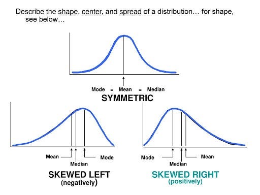
Skewness

• 📺 Skewness Video

• Symmetric: Mode = Median = Mean
• Positively skewed: Mean > Median > Mode
• Negatively skewed: Mean < Median < Mode

2.2 Measures of Dispersion

• [[Range, Variance, Standard Deviation, The Coefficient of Variation]]

• [[The Interquartile Range, A Box-and-Whisker Plot]]

Range

$\text{Range} = x_{\text{max}} - x_{\text{min}}$

Variance and Standard Deviation

• Sample Variance
  $s^2 = \frac{\sum (x - \bar{x})^2}{n - 1} = \frac{\sum x^2 - \frac{(\sum x)^2}{n}}{n - 1}$

• Sample Standard Deviation
  $s = \sqrt{s^2}$

Coefficient of Variation

• A normalized measure of dispersion:
  $\text{CV} = \frac{s}{\bar{x}} \times 100$

Interquartile Range (IQR)

x_min ─── Q₁ ─── Q₂ (Median) ─── Q₃ ─── x_max
       25%    25%             25%    25%

$IQR = Q_3 - Q_1$

Box-and-Whisker Plot

• Box plot includes: min, max, lower quartile (Q1), median (Q2), upper quartile (Q3).
• Whiskers:
  • Lower whisker: larger of lower limit or minimum value.
  • Upper whisker: smaller of upper limit or maximum value.

---

3. Basic Probability

3.1 Sample Space & Events

Concepts

• Sample Space ($S$): Set of all possible outcomes of the experiment.
  • $P(S) = 1$
• Event ($E$): A subset of $S$
• Complement of Event $E$ ($\overline{E}$ or $E^c$): Event not in $E$ $$P(\overline{E}) = 1 - P(E)$$

AND, OR

• AND ($E \cap F$): Both $E$ and $F$ occur
• OR ($E \cup F$): $E$, $F$, or both occur

Mutually Exclusive and Subset

• Mutually Exclusive: $E \cap F = \emptyset$
• Subset: $E \subseteq F$

Axioms of Probability

1. $0 \leq P(E) \leq 1$
2. $P(S) = 1$
3. For mutually exclusive events: $$P(E_1 \cup E_2 \cup ... \cup E_n) = P(E_1) + P(E_2) + ... + P(E_n)$$

Algebra of Events

• Complement Rule: $$P(\overline{E}) = 1 - P(E)$$
• Addition Rule: $$P(E \cup F) = P(E) + P(F) - P(E \cap F)$$

Extended Concepts

• Mutually Exclusive: Cannot occur together (e.g., coin toss: head or tail)
• Independent: One does not affect the other (e.g., YouTube like and share)

Probability of $A$ and not $B$

• $P(A \text{ and } \overline{B}) = P(A) - P(A \cap B)$

3.2 Conditional Probability

• Conditional probability: $$P(A | B) = \frac{P(A \cap B)}{P(B)}$$

Total Probability Rule

• If $B_1, B_2, ..., B_n$ are mutually exclusive and exhaustive events: $$P(A) = \sum_{i=1}^{n} P(A|B_i)P(B_i)$$

3.3 Independent Events

• $E$ and $F$ are independent if: $$P(E \cap F) = P(E)P(F)$$
• Check independence: $$P(E) = P(E|F) \iff P(E \cap F) = P(E)P(F)$$
• Independent ≠ Mutually Exclusive

3.4 Bayes' Theorem

• Formula: $$P(A|B) = \frac{P(B|A) \cdot P(A)}{P(B)}$$

Reference

• Bayes' Theorem Video

---

4. Discrete Random Variables

4.1 Introduction to Random Variables

Concept

• Sample Space (S): Set of all possible outcomes of a statistical experiment.
• Element/Sample point: Each outcome that belongs to the sample space.
• Random Variable: A function applied to sample space and its elements to generate a range of values used for probability calculation.

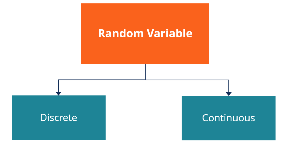
4.2 Discrete and Continuous Random Variables

Concept

• Discrete Sample Space: Countable outcomes.
  • Discrete Random Variable: A random variable defined over a discrete sample space.
• Continuous Sample Space: Uncountable outcomes.
  • Continuous Random Variable: A random variable defined over a continuous sample space.

4.3 The Binomial and Poisson Distributions

Binomial Distribution

Conditions

• Experiment consists of $n$ trials.
• Each trial has two possible outcomes (success/failure).
• Probability of success $p$ remains constant.
• Trials are independent.

Distribution

$X \sim B(n, p)$

• Formula:
  $P_r = \binom{n}{r} p^r q^{n-r}$
  where $q = 1 - p$

• Expected Value:
  $E(X) = n \cdot p$

• Variance:
  $Var(X) = \sigma^2 = n \cdot p \cdot q$

Poisson Distribution

Conditions

• Describes number of events over an interval (time, area, volume).
• Occurrences happen:
  • Randomly
  • Independently
  • At a constant average rate

Distribution

$X \sim Po(\lambda)$

• Formula:
  $P(X = x) = \frac{e^{-\lambda} \lambda^x}{x!}, \quad \lambda > 0$

• Expected Value and Variance:
  $E(X) = \mu = \lambda, \quad Var(X) = \lambda$

• Probability of $r$ occurrences:
  $P(X = r) = \frac{e^{-\lambda} \lambda^r}{r!}$
  $E(X = r) = n \cdot P(X = r)$

Notes:

• Discrete values
• No upper bound
• Mean and variance are approximately equal